<?xml version="1.0" encoding="utf-8"?><feed xmlns="http://www.w3.org/2005/Atom" xml:lang="en"><generator uri="https://jekyllrb.com/" version="4.4.1">Jekyll</generator><link href="https://blogs.gruheshkurra.com/feed.xml" rel="self" type="application/atom+xml" /><link href="https://blogs.gruheshkurra.com/" rel="alternate" type="text/html" hreflang="en" /><updated>2026-09-08T16:50:43+00:00</updated><id>https://blogs.gruheshkurra.com/feed.xml</id><title type="html">Gruhesh Sri Sai Karthik Kurra</title><subtitle>Deep-dive notes on AI, machine learning, and LLMs: full derivations, worked numbers, and code that runs.</subtitle><author><name>Gruhesh Sri Sai Karthik Kurra</name><email>gruheshkurra2@gmail.com</email></author><entry><title type="html">Convolutional Neural Networks: CNN Math Explained</title><link href="https://blogs.gruheshkurra.com/blog/convolutional-neural-networks-explained/" rel="alternate" type="text/html" title="Convolutional Neural Networks: CNN Math Explained" /><published>2026-09-08T12:30:00+00:00</published><updated>2026-09-08T12:30:00+00:00</updated><id>https://blogs.gruheshkurra.com/blog/convolutional-neural-networks-explained</id><content type="html" xml:base="https://blogs.gruheshkurra.com/blog/convolutional-neural-networks-explained/"><![CDATA[<p>A convolutional neural network learns small filters and applies each filter across an image. Each output is a weighted sum of a local patch. Reusing the weights gives the network a useful assumption: a pattern worth detecting in one place may also be worth detecting elsewhere.</p>

<p>I want to keep the arithmetic visible here. One small image, one filter, every output, then a backward pass that changes the filter. The larger architecture grows from those operations.</p>

<blockquote>
  <p>[!NOTE]
The prerequisites are a dot product and the chain rule. The earlier posts on <a href="/blog/essence-of-linear-algebra/">linear algebra</a> and <a href="/blog/build-autograd-from-scratch/">backpropagation</a> cover those. A dot product multiplies matching entries and adds them; the chain rule multiplies derivatives along a path and adds contributions from different paths.</p>
</blockquote>

<h2 id="what-does-a-cnn-do-to-an-image">What does a CNN do to an image?</h2>

<p>Here is a small classifier I will use for the shape calculations. Its widths are chosen for this example; they are not measurements from a trained model. Both convolutions use stride one, dilation one, and a learned bias per filter.</p>

<pre><code class="language-mermaid">flowchart TD
  X["RGB image: 3 × 32 × 32"] --&gt; C1["3 × 3 convolution: 8 filters, padding 1"]
  C1 --&gt; A1["ReLU: 8 × 32 × 32"]
  A1 --&gt; P["2 × 2 max pooling, stride 2: 8 × 16 × 16"]
  P --&gt; C2["3 × 3 convolution: 16 filters, padding 1"]
  C2 --&gt; A2["ReLU: 16 × 16 × 16"]
  A2 --&gt; G["Global average pooling: 16 numbers"]
  G --&gt; F["Linear classifier: 10 logits"]
  F --&gt; L["Softmax probabilities and cross-entropy loss"]
</code></pre>

<p>An image is a tensor, an array with several axes. I use channel-first notation: channels, height, width. A batch adds an axis in front.</p>

<table>
  <thead>
    <tr>
      <th>Symbol</th>
      <th>Meaning</th>
      <th>Shape or range</th>
    </tr>
  </thead>
  <tbody>
    <tr>
      <td>$N$</td>
      <td>Images in a batch</td>
      <td>Positive integer</td>
    </tr>
    <tr>
      <td>$C_{\mathrm{in}}, C_{\mathrm{out}}$</td>
      <td>Input and output channels</td>
      <td>Positive integers</td>
    </tr>
    <tr>
      <td>$H,W$</td>
      <td>Input height and width</td>
      <td>Positive integers</td>
    </tr>
    <tr>
      <td>$k_h,k_w$</td>
      <td>Filter height and width</td>
      <td>Positive integers</td>
    </tr>
    <tr>
      <td>$X$</td>
      <td>Input batch</td>
      <td>$N\times C_{\mathrm{in}}\times H\times W$</td>
    </tr>
    <tr>
      <td>$K$</td>
      <td>Learned filter weights</td>
      <td>$C_{\mathrm{out}}\times C_{\mathrm{in}}\times k_h\times k_w$</td>
    </tr>
    <tr>
      <td>$b$</td>
      <td>One learned bias per output channel</td>
      <td>$C_{\mathrm{out}}$</td>
    </tr>
    <tr>
      <td>$Z,A$</td>
      <td>Values before and after activation</td>
      <td>$N\times C_{\mathrm{out}}\times H_{\mathrm{out}}\times W_{\mathrm{out}}$</td>
    </tr>
  </tbody>
</table>

<p>RGB provides three input channels. Eight filters produce eight output channels, also called feature maps. Each filter spans all three RGB channels. The network sums those channel contributions to produce one value at each output position.<sup id="fnref:conv2d"><a href="#fn:conv2d" class="footnote" rel="footnote" role="doc-noteref">1</a></sup></p>

<p>Pooling reduces spatial size. ReLU changes values without changing shape. The last linear layer produces one raw score, or logit, per class.</p>

<h2 id="how-does-a-convolution-work">How does a convolution work?</h2>

<p>Start with one grayscale image, one filter, stride one, and no padding. Omit the batch and channel axes. The output at row $i$, column $j$ is</p>

<div class="kdmath">$$
Z_{i,j}=b+\sum_{u=0}^{k_h-1}\sum_{v=0}^{k_w-1}K_{u,v}X_{i+u,j+v}.
$$</div>

<p>The indices $u,v$ select positions inside the filter. The indices $i,j$ select its placement on the image. Move the filter, multiply matching entries, sum, and add the same bias.</p>

<h3 id="one-complete-numerical-convolution">One complete numerical convolution</h3>

<p>Given a $3\times3$ input, a $2\times2$ filter, and scalar bias $b=0$:</p>

<div class="kdmath">$$
X=\begin{bmatrix}1&2&0\\0&1&3\\2&1&0\end{bmatrix},
\qquad
K=\begin{bmatrix}1&0\\0&-1\end{bmatrix}.
$$</div>

<p>Find the $2\times2$ output. For the top-left patch, the four products are</p>

<div class="kdmath">$$
\begin{aligned}
1\cdot1&=1,\\
0\cdot2&=0,\\
0\cdot0&=0,\\
(-1)\cdot1&=-1.
\end{aligned}
$$</div>

<p>Add them, then add the bias:</p>

<div class="kdmath">$$
\begin{aligned}
1+0&=1,\\
1+0&=1,\\
1+(-1)&=0,\\
Z_{0,0}&=0+0=0.
\end{aligned}
$$</div>

<p>The remaining placements use the same four weights:</p>

<table>
  <thead>
    <tr>
      <th>Output</th>
      <th>Matching products</th>
      <th>Sum, then bias</th>
      <th style="text-align: right">Result</th>
    </tr>
  </thead>
  <tbody>
    <tr>
      <td>$Z_{0,0}$</td>
      <td>$1\cdot1+0\cdot2+0\cdot0-1\cdot1$</td>
      <td>$1+0+0-1+0$</td>
      <td style="text-align: right">0</td>
    </tr>
    <tr>
      <td>$Z_{0,1}$</td>
      <td>$1\cdot2+0\cdot0+0\cdot1-1\cdot3$</td>
      <td>$2+0+0-3+0$</td>
      <td style="text-align: right">-1</td>
    </tr>
    <tr>
      <td>$Z_{1,0}$</td>
      <td>$1\cdot0+0\cdot1+0\cdot2-1\cdot1$</td>
      <td>$0+0+0-1+0$</td>
      <td style="text-align: right">-1</td>
    </tr>
    <tr>
      <td>$Z_{1,1}$</td>
      <td>$1\cdot1+0\cdot3+0\cdot1-1\cdot0$</td>
      <td>$1+0+0+0+0$</td>
      <td style="text-align: right">1</td>
    </tr>
  </tbody>
</table>

<div class="kdmath">$$
Z=\begin{bmatrix}0&-1\\-1&1\end{bmatrix}.
$$</div>

<p>Check: a two-cell-wide filter fits at two positions along each three-cell axis. The output has four values. This particular filter measures the top-left value minus the bottom-right value of each patch.</p>

<h3 id="is-this-convolution-or-cross-correlation">Is this convolution or cross-correlation?</h3>

<p>The operation above is cross-correlation. Mathematical convolution flips the kernel along both spatial axes. CNN libraries commonly keep the unflipped operation and call the layer convolution.<sup id="fnref:book"><a href="#fn:book" class="footnote" rel="footnote" role="doc-noteref">2</a></sup></p>

<p>For the numerical kernel, a flip gives</p>

<div class="kdmath">$$
K_{\mathrm{flipped}}=\begin{bmatrix}-1&0\\0&1\end{bmatrix}.
$$</div>

<p>On the top-right patch, that produces $-2+3=1$, while the unflipped filter produced $-1$. The convention changes a calculation with fixed weights. With unrestricted learned weights, either orientation can represent the same filters. I use the unflipped convention throughout.</p>

<h2 id="what-do-stride-padding-and-dilation-change">What do stride, padding, and dilation change?</h2>

<p>Stride $s$ is the step between filter placements. Padding $p$ adds cells on each side; here those cells are zero. Dilation $d$ is the spacing between sampled filter entries. All three affect the output size.</p>

<p>For one spatial axis, let $n$ be the input length and $k$ the number of filter entries. The effective filter span is</p>

<div class="kdmath">$$
k_{\mathrm{eff}}=d(k-1)+1.
$$</div>

<p>The padded input has length $n+2p$. A filter whose starting coordinate is $t$ fits if</p>

<div class="kdmath">$$
\begin{aligned}
t+k_{\mathrm{eff}}&\leq n+2p,\\
t&\leq n+2p-k_{\mathrm{eff}}.
\end{aligned}
$$</div>

<p>Starts occur at $0,s,2s,\ldots$. Count those positions, including the first:</p>

<div class="kdmath">$$
n_{\mathrm{out}}=\left\lfloor\frac{n+2p-d(k-1)-1}{s}\right\rfloor+1.
$$</div>

<p>Apply this separately to height and width. This formula assumes symmetric padding, positive integer stride and dilation, and an effective kernel that fits the padded input.<sup id="fnref:conv2d:1"><a href="#fn:conv2d" class="footnote" rel="footnote" role="doc-noteref">1</a></sup></p>

<p>For $n=32$, $k=3$, $p=1$, $d=1$, and $s=2$:</p>

<div class="kdmath">$$
\begin{aligned}
k_{\mathrm{eff}}&=1(3-1)+1=3,\\
n+2p&=32+2=34,\\
34-3&=31,\\
31/2&=15.5,\\
\lfloor15.5\rfloor&=15,\\
n_{\mathrm{out}}&=15+1=16.
\end{aligned}
$$</div>

<p>The final unused position is allowed. There is no requirement that the division produce an integer.</p>

<table>
  <thead>
    <tr>
      <th style="text-align: right">Input axis</th>
      <th style="text-align: right">Kernel</th>
      <th style="text-align: right">Padding per side</th>
      <th style="text-align: right">Stride</th>
      <th style="text-align: right">Dilation</th>
      <th style="text-align: right">Effective span</th>
      <th style="text-align: right">Output axis</th>
    </tr>
  </thead>
  <tbody>
    <tr>
      <td style="text-align: right">32</td>
      <td style="text-align: right">3</td>
      <td style="text-align: right">0</td>
      <td style="text-align: right">1</td>
      <td style="text-align: right">1</td>
      <td style="text-align: right">3</td>
      <td style="text-align: right">30</td>
    </tr>
    <tr>
      <td style="text-align: right">32</td>
      <td style="text-align: right">3</td>
      <td style="text-align: right">1</td>
      <td style="text-align: right">1</td>
      <td style="text-align: right">1</td>
      <td style="text-align: right">3</td>
      <td style="text-align: right">32</td>
    </tr>
    <tr>
      <td style="text-align: right">32</td>
      <td style="text-align: right">3</td>
      <td style="text-align: right">1</td>
      <td style="text-align: right">2</td>
      <td style="text-align: right">1</td>
      <td style="text-align: right">3</td>
      <td style="text-align: right">16</td>
    </tr>
    <tr>
      <td style="text-align: right">32</td>
      <td style="text-align: right">3</td>
      <td style="text-align: right">2</td>
      <td style="text-align: right">1</td>
      <td style="text-align: right">2</td>
      <td style="text-align: right">5</td>
      <td style="text-align: right">32</td>
    </tr>
  </tbody>
</table>

<p>The dilated filter still has three entries per axis. It samples offsets $0,2,4$ across a five-cell span. A two-dimensional $3\times3$ dilated filter has nine spatial weights, not twenty-five.</p>

<p>For completeness, the channel-aware forward equation for one image is</p>

<div class="kdmath">$$
Z_{o,i,j}=b_o+
\sum_{c=0}^{C_{\mathrm{in}}-1}
\sum_{u=0}^{k_h-1}\sum_{v=0}^{k_w-1}
K_{o,c,u,v}\,
\widetilde X_{c,\,i s_h+u d_h,\,j s_w+v d_w}.
$$</div>

<p>Here $o$ selects the output channel, $c$ selects the input channel, and $\widetilde X$ is the already padded image. Subscripts $h,w$ allow separate vertical and horizontal settings. This is ordinary convolution with all input channels connected to every output channel, also called <code class="language-plaintext highlighter-rouge">groups=1</code>.</p>

<h2 id="why-does-weight-sharing-save-parameters">Why does weight sharing save parameters?</h2>

<p>One filter has $C_{\mathrm{in}}k_hk_w$ weights and one bias. There are $C_{\mathrm{out}}$ filters, so</p>

<div class="kdmath">$$
P_{\mathrm{conv}}=C_{\mathrm{out}}(C_{\mathrm{in}}k_hk_w+1).
$$</div>

<p>The image height and width are absent. A larger image uses the weights more times; it does not add weights to this layer.</p>

<p>For the first layer of our classifier:</p>

<div class="kdmath">$$
\begin{aligned}
\text{spatial entries}&=3\cdot3=9,\\
\text{weights per filter}&=3\cdot9=27,\\
\text{parameters per filter}&=27+1=28,\\
P_{\mathrm{conv}}&=8\cdot28=224.
\end{aligned}
$$</div>

<p>It produces $8\cdot32\cdot32=8{,}192$ output values from $3\cdot32\cdot32=3{,}072$ input values. Compare layers producing that same number of outputs:</p>

<table>
  <thead>
    <tr>
      <th>Connection pattern</th>
      <th>Parameters with bias</th>
      <th style="text-align: right">Computed total</th>
    </tr>
  </thead>
  <tbody>
    <tr>
      <td>Dense: every output sees every input</td>
      <td>$8{,}192(3{,}072+1)$</td>
      <td style="text-align: right">25,174,016</td>
    </tr>
    <tr>
      <td>Local: a separate 27-weight filter at each output</td>
      <td>$8{,}192(27+1)$</td>
      <td style="text-align: right">229,376</td>
    </tr>
    <tr>
      <td>Convolution: eight filters reused at every location</td>
      <td>$8(27+1)$</td>
      <td style="text-align: right">224</td>
    </tr>
  </tbody>
</table>

<p>The local row counts all patch slots, including slots touching padded zeros. The dense layer can represent functions this convolution cannot. The saving comes from restricting the connections and requiring weights at different positions to match.</p>

<p>There is a linear-algebra view of the same restriction. Flatten a one-dimensional input $x=[x_0,x_1,x_2]^\top$ and apply weights $a,b$ with no bias:</p>

<div class="kdmath">$$
\begin{bmatrix}y_0\\y_1\end{bmatrix}
=\begin{bmatrix}a&b&0\\0&a&b\end{bmatrix}
\begin{bmatrix}x_0\\x_1\\x_2\end{bmatrix}.
$$</div>

<p>The $2\times3$ matrix contains repeated weights and zeros. With $a=1$, $b=-1$, and $x=[1,2,4]^\top$, its rows give $y_0=1-2=-1$ and $y_1=2-4=-2$. A spatial convolution is a structured linear map. Adding a bias makes it affine.</p>

<h2 id="why-add-relu-and-pooling">Why add ReLU and pooling?</h2>

<p>ReLU, the rectified linear unit, acts on each scalar:</p>

<div class="kdmath">$$
A_{i,j}=\max(0,Z_{i,j}).
$$</div>

<p>Our numerical convolution becomes</p>

<div class="kdmath">$$
\begin{bmatrix}0&-1\\-1&1\end{bmatrix}
\quad\longrightarrow\quad
\begin{bmatrix}0&0\\0&1\end{bmatrix}.
$$</div>

<p>Without nonlinear operations, a stack of affine layers remains one affine map. If $W_1,W_2$ are compatible matrices and $b_1,b_2$ their biases, expand two layers:</p>

<div class="kdmath">$$
\begin{aligned}
h&=W_1x+b_1,\\
y&=W_2h+b_2,\\
y&=W_2(W_1x+b_1)+b_2,\\
y&=(W_2W_1)x+(W_2b_1+b_2).
\end{aligned}
$$</div>

<p>ReLU makes which entries pass through depend on the input. The resulting network is piecewise affine rather than one affine function everywhere.</p>

<p>A $2\times2$ max pool with stride two selects the largest value in each non-overlapping window. Average pooling takes the mean. Applied to the activated patch above:</p>

<div class="kdmath">$$
\begin{aligned}
\operatorname{maxpool}(A)&=\max(0,0,0,1)=1,\\
\operatorname{avgpool}(A)&=(0+0+0+1)/4=0.25.
\end{aligned}
$$</div>

<p>Both turn this $2\times2$ map into $1\times1$ and add no learned parameters. They discard different information. Max pooling keeps the largest response; averaging keeps its contribution relative to the whole window.</p>

<p>Global average pooling takes the mean of an entire channel. For a map of height $h$ and width $w$, its channel-$c$ output is</p>

<div class="kdmath">$$
g_c=\frac{1}{hw}\sum_{i=0}^{h-1}\sum_{j=0}^{w-1}A_{c,i,j}.
$$</div>

<p>In the classifier, each of the sixteen $16\times16$ maps becomes one number. The final dense layer therefore needs $10(16+1)=170$ parameters. Flattening those maps first would give $16\cdot16\cdot16=4{,}096$ inputs and $10(4{,}096+1)=40{,}970$ parameters. Averaging saves parameters but removes explicit spatial layout from the classifier input.</p>

<h2 id="how-does-a-small-filter-see-a-larger-region">How does a small filter see a larger region?</h2>

<p>A receptive field is the region of the original input that can affect a particular feature. Later filters read earlier features, so their input coverage grows with depth.<sup id="fnref:receptive"><a href="#fn:receptive" class="footnote" rel="footnote" role="doc-noteref">3</a></sup></p>

<p>For a sequential stack, track $r_\ell$, the receptive-field width after layer $\ell$, and $j_\ell$, the distance in original-input pixels between neighboring features. Start with $r_0=j_0=1$. With effective kernel span $k_{\mathrm{eff},\ell}$ and stride $s_\ell$:</p>

<div class="kdmath">$$
\begin{aligned}
r_\ell&=r_{\ell-1}+(k_{\mathrm{eff},\ell}-1)j_{\ell-1},\\
j_\ell&=s_\ell j_{\ell-1}.
\end{aligned}
$$</div>

<p>A filter adds one previous jump for each extra sampled position when dilation is one. Dilation stretches that span. Apply the equations per axis to the example architecture:</p>

<table>
  <thead>
    <tr>
      <th>Layer</th>
      <th>Receptive-field calculation</th>
      <th style="text-align: right">Width $r$</th>
      <th style="text-align: right">Jump $j$</th>
    </tr>
  </thead>
  <tbody>
    <tr>
      <td>Input</td>
      <td>Initial pixel</td>
      <td style="text-align: right">1</td>
      <td style="text-align: right">1</td>
    </tr>
    <tr>
      <td>$3\times3$ convolution, stride 1</td>
      <td>$1+(3-1)\cdot1$</td>
      <td style="text-align: right">3</td>
      <td style="text-align: right">1</td>
    </tr>
    <tr>
      <td>ReLU</td>
      <td>Pointwise; no added coverage</td>
      <td style="text-align: right">3</td>
      <td style="text-align: right">1</td>
    </tr>
    <tr>
      <td>$2\times2$ pool, stride 2</td>
      <td>$3+(2-1)\cdot1$</td>
      <td style="text-align: right">4</td>
      <td style="text-align: right">2</td>
    </tr>
    <tr>
      <td>$3\times3$ convolution, stride 1</td>
      <td>$4+(3-1)\cdot2$</td>
      <td style="text-align: right">8</td>
      <td style="text-align: right">2</td>
    </tr>
  </tbody>
</table>

<p>Each feature before global pooling can depend on an $8\times8$ region. At image edges, part of that region may be padding. This is theoretical coverage; learned weights and activation gates determine which inputs influence a particular prediction.</p>

<h2 id="are-cnns-translation-invariant">Are CNNs translation invariant?</h2>

<p>Translation equivariance means shifting the input shifts the feature map by the corresponding amount. Translation invariance means the output stays the same. These are different properties.</p>

<p>The weight-sharing equation explains equivariance. Use one dimension, stride one, and an infinite grid to avoid boundary issues. Define a shift by integer $a$ as $(T_a x)[i]=x[i-a]$. Let $F$ be cross-correlation with fixed kernel $k[u]$:</p>

<div class="kdmath">$$
\begin{aligned}
F(x)[i]&=\sum_u k[u]x[i+u],\\
F(T_a x)[i]&=\sum_u k[u]x[i+u-a],\\
F(x)[i-a]&=\sum_u k[u]x[(i-a)+u],\\
F(T_a x)&=T_aF(x).
\end{aligned}
$$</div>

<p>For example, with $k=[1,-1]$, a value $5$ at input position 2 and zeros elsewhere produces $-5$ at output position 1 and $5$ at position 2. Move that input value to position 3: the outputs move to positions 2 and 3. Their values do not change.</p>

<p>Finite-image boundaries and subsampling need more care. Here is a counterexample to the claim that max pooling guarantees invariance. Use width-two max pooling with stride two, and circularly shift a four-entry input one place right:</p>

<div class="kdmath">$$
\begin{aligned}
x&=[1,2,3,4], &\operatorname{pool}(x)&=[2,4],\\
T_1x&=[4,1,2,3], &\operatorname{pool}(T_1x)&=[4,3].
\end{aligned}
$$</div>

<p>The pooled values changed. The shift changed which values shared a window. Zhang’s work on antialiased CNNs studies this sensitivity to downsampling.<sup id="fnref:shift"><a href="#fn:shift" class="footnote" rel="footnote" role="doc-noteref">4</a></sup></p>

<p>Global averaging is invariant to a permutation of an unchanged set of feature values. An image shift that introduces padding, crops content, or changes downsampled features can change that set. A CNN classifier therefore has no blanket guarantee of translation invariance.</p>

<h2 id="what-objective-trains-a-cnn-classifier">What objective trains a CNN classifier?</h2>

<p>For our ten-class model, global pooling produces $g\in\mathbb R^{16}$. The classifier has $V\in\mathbb R^{10\times16}$ and bias $a\in\mathbb R^{10}$:</p>

<div class="kdmath">$$
\ell=Vg+a.
$$</div>

<p>The logit vector $\ell$ has ten entries. For $M$ mutually exclusive classes, softmax converts logits to probabilities $p_j$. If the correct class is $t$, cross-entropy loss is</p>

<div class="kdmath">$$
p_j=\frac{e^{\ell_j}}{\sum_{q=1}^{M}e^{\ell_q}},
\qquad L=-\log p_t.
$$</div>

<p>Use two logits $[\log2,0]$ and correct class $t=1$ to make one prediction by hand:</p>

<div class="kdmath">$$
\begin{aligned}
e^{\log2}&=2, &e^0&=1,\\
2+1&=3, &p&=[2/3,1/3],\\
L&=-\log(2/3)=\log(3/2)\approx0.405465.
\end{aligned}
$$</div>

<p>The probabilities sum to one. The loss is positive because the correct class has probability below one; the decimal is rounded to six places.</p>

<p>To differentiate with respect to logit $\ell_j$, expand the log probability first:</p>

<div class="kdmath">$$
\begin{aligned}
L&=-\ell_t+\log\sum_q e^{\ell_q},\\
\frac{\partial L}{\partial\ell_j}
&=-\mathbf1[j=t]+\frac{1}{\sum_q e^{\ell_q}}e^{\ell_j},\\
\frac{\partial L}{\partial\ell_j}&=p_j-\mathbf1[j=t].
\end{aligned}
$$</div>

<p>The indicator $\mathbf1[j=t]$ equals one for the correct class and zero otherwise. The two-logit example gives gradients $[-1/3,1/3]$. Gradient descent raises the correct logit and lowers the other one. The <a href="/blog/cross-entropy-loss-explained/">cross-entropy post</a> follows this objective in more detail.</p>

<h2 id="how-does-backpropagation-update-a-shared-filter">How does backpropagation update a shared filter?</h2>

<p>Let $\delta_{o,i,j}=\partial L/\partial Z_{o,i,j}$ be the gradient arriving at a convolution’s output before activation. For valid, stride-one cross-correlation on one image, differentiate with respect to one weight:</p>

<div class="kdmath">$$
\begin{aligned}
\frac{\partial Z_{o,i,j}}{\partial K_{o,c,u,v}}&=X_{c,i+u,j+v},\\
\frac{\partial L}{\partial K_{o,c,u,v}}
&=\sum_{i,j}\frac{\partial L}{\partial Z_{o,i,j}}
\frac{\partial Z_{o,i,j}}{\partial K_{o,c,u,v}},\\
\frac{\partial L}{\partial K_{o,c,u,v}}
&=\sum_{i,j}\delta_{o,i,j}X_{c,i+u,j+v}.
\end{aligned}
$$</div>

<p>The same weight helped produce many output values, so it receives a contribution from each use. Biases obey the same rule:<sup id="fnref:gradients"><a href="#fn:gradients" class="footnote" rel="footnote" role="doc-noteref">5</a></sup></p>

<div class="kdmath">$$
\frac{\partial L}{\partial b_o}=\sum_{i,j}\delta_{o,i,j}.
$$</div>

<p>For a batch, also sum over images. If the objective averages examples, that normalization is already present in $\delta$.</p>

<p>The input gradient adds contributions from every output window that used the input pixel. For input row $r$, column $s$:</p>

<div class="kdmath">$$
\frac{\partial L}{\partial X_{c,r,s}}
=\sum_o\sum_{u,v}K_{o,c,u,v}\,\delta_{o,r-u,s-v},
$$</div>

<p>where out-of-range $\delta$ entries are zero. The subtraction in the indices comes from solving $r=i+u$ and $s=j+v$ for the output position.</p>

<p>ReLU supplies a gate before these sums. If $G=\partial L/\partial A$ is the arriving gradient, then</p>

<div class="kdmath">$$
\delta_{i,j}=G_{i,j}\mathbf1[Z_{i,j}>0].
$$</div>

<p>At zero, ReLU has no unique derivative; taking the gradient as zero is a common convention. A max-pooling backward pass routes the gradient to the selected maximum. Average pooling spreads it equally across the window. For a unique maximum in a $2\times2$ window and incoming gradient $4$, max pooling sends $4$ to that entry; average pooling sends $1$ to each of the four entries. Tied maxima need a defined selection or subgradient convention.</p>

<h3 id="one-full-gradient-descent-step">One full gradient-descent step</h3>

<p>I will isolate the convolution and ReLU so every learned value fits on paper. Use the same $X$ and $K$ from the forward example, change the initial bias to $b=2$, and choose a $2\times2$ target map $Y$. This is a small regression exercise with squared error, separate from the classification objective above.</p>

<div class="kdmath">$$
X=\begin{bmatrix}1&2&0\\0&1&3\\2&1&0\end{bmatrix},\quad
K=\begin{bmatrix}1&0\\0&-1\end{bmatrix},\quad
Y=\begin{bmatrix}1&0\\0&2\end{bmatrix}.
$$</div>

<p>Find the gradients of all four weights and the bias, update them with learning rate $\eta=0.01$, and recompute the loss.</p>

<p>Add two to every entry of the earlier convolution output:</p>

<div class="kdmath">$$
Z=\begin{bmatrix}0+2&-1+2\\-1+2&1+2\end{bmatrix}
=\begin{bmatrix}2&1\\1&3\end{bmatrix},\qquad
A=\operatorname{ReLU}(Z)=\begin{bmatrix}2&1\\1&3\end{bmatrix}.
$$</div>

<p>All entries are positive, so all four ReLU derivatives are one. Define a summed loss, with no division by the four outputs:</p>

<div class="kdmath">$$
L=\frac12\sum_{i,j}(A_{i,j}-Y_{i,j})^2.
$$</div>

<p>Subtract the target and square each residual:</p>

<div class="kdmath">$$
\begin{aligned}
A-Y&=\begin{bmatrix}2-1&1-0\\1-0&3-2\end{bmatrix}
=\begin{bmatrix}1&1\\1&1\end{bmatrix},\\
L&=\tfrac12(1^2+1^2+1^2+1^2)=2.
\end{aligned}
$$</div>

<p>The outer derivative of $\frac12 e^2$ with respect to residual $e$ is $e$. The derivative of $e=A-Y$ with respect to $A$ is one. Multiply those derivatives and the ReLU gate:</p>

<div class="kdmath">$$
\delta=(A-Y)\odot\mathbf1[Z>0]
=\begin{bmatrix}1&1\\1&1\end{bmatrix},
$$</div>

<p>where $\odot$ means entry-by-entry multiplication. Each shared weight accumulates four contributions, in output order $(0,0),(0,1),(1,0),(1,1)$:</p>

<table>
  <thead>
    <tr>
      <th>Parameter</th>
      <th>Gradient contributions</th>
      <th style="text-align: right">Sum</th>
    </tr>
  </thead>
  <tbody>
    <tr>
      <td>$K_{0,0}$</td>
      <td>$1\cdot1+1\cdot2+1\cdot0+1\cdot1$</td>
      <td style="text-align: right">4</td>
    </tr>
    <tr>
      <td>$K_{0,1}$</td>
      <td>$1\cdot2+1\cdot0+1\cdot1+1\cdot3$</td>
      <td style="text-align: right">6</td>
    </tr>
    <tr>
      <td>$K_{1,0}$</td>
      <td>$1\cdot0+1\cdot1+1\cdot2+1\cdot1$</td>
      <td style="text-align: right">4</td>
    </tr>
    <tr>
      <td>$K_{1,1}$</td>
      <td>$1\cdot1+1\cdot3+1\cdot1+1\cdot0$</td>
      <td style="text-align: right">5</td>
    </tr>
    <tr>
      <td>$b$</td>
      <td>$1+1+1+1$</td>
      <td style="text-align: right">4</td>
    </tr>
  </tbody>
</table>

<p>Check the gradient shapes: $\nabla_KL$ is $2\times2$, matching $K$; $\partial L/\partial b$ is a scalar. For the center input pixel, all four output windows contribute:</p>

<div class="kdmath">$$
\frac{\partial L}{\partial X_{1,1}}
=1(-1)+1(0)+1(0)+1(1)=0.
$$</div>

<p>Some paths cancel. The filter gradients still need all four paths.</p>

<p>Apply $\theta_{\mathrm{new}}=\theta-\eta\nabla_\theta L$ to each learned parameter:</p>

<table>
  <thead>
    <tr>
      <th>Parameter</th>
      <th>Learning rate × gradient</th>
      <th>Old value − update</th>
      <th style="text-align: right">New value</th>
    </tr>
  </thead>
  <tbody>
    <tr>
      <td>$K_{0,0}$</td>
      <td>$0.01\cdot4=0.04$</td>
      <td>$1-0.04$</td>
      <td style="text-align: right">0.96</td>
    </tr>
    <tr>
      <td>$K_{0,1}$</td>
      <td>$0.01\cdot6=0.06$</td>
      <td>$0-0.06$</td>
      <td style="text-align: right">-0.06</td>
    </tr>
    <tr>
      <td>$K_{1,0}$</td>
      <td>$0.01\cdot4=0.04$</td>
      <td>$0-0.04$</td>
      <td style="text-align: right">-0.04</td>
    </tr>
    <tr>
      <td>$K_{1,1}$</td>
      <td>$0.01\cdot5=0.05$</td>
      <td>$-1-0.05$</td>
      <td style="text-align: right">-1.05</td>
    </tr>
    <tr>
      <td>$b$</td>
      <td>$0.01\cdot4=0.04$</td>
      <td>$2-0.04$</td>
      <td style="text-align: right">1.96</td>
    </tr>
  </tbody>
</table>

<p>Recompute every output using those new values:</p>

<table>
  <thead>
    <tr>
      <th>Output</th>
      <th>Products plus bias</th>
      <th style="text-align: right">Result</th>
    </tr>
  </thead>
  <tbody>
    <tr>
      <td>$Z^{\prime}_{0,0}$</td>
      <td>$0.96-0.12+0-1.05+1.96$</td>
      <td style="text-align: right">1.75</td>
    </tr>
    <tr>
      <td>$Z^{\prime}_{0,1}$</td>
      <td>$1.92+0-0.04-3.15+1.96$</td>
      <td style="text-align: right">0.69</td>
    </tr>
    <tr>
      <td>$Z^{\prime}_{1,0}$</td>
      <td>$0-0.06-0.08-1.05+1.96$</td>
      <td style="text-align: right">0.77</td>
    </tr>
    <tr>
      <td>$Z^{\prime}_{1,1}$</td>
      <td>$0.96-0.18-0.04+0+1.96$</td>
      <td style="text-align: right">2.70</td>
    </tr>
  </tbody>
</table>

<p>All outputs remain positive, so ReLU leaves them unchanged. The new residuals and loss are</p>

<div class="kdmath">$$
\begin{aligned}
A'-Y&=\begin{bmatrix}0.75&0.69\\0.77&0.70\end{bmatrix},\\
0.75^2&=0.5625,\\
0.69^2&=0.4761,\\
0.77^2&=0.5929,\\
0.70^2&=0.4900,\\
0.5625+0.4761&=1.0386,\\
1.0386+0.5929&=1.6315,\\
1.6315+0.4900&=2.1215,\\
L'&=\tfrac12\cdot2.1215=1.06075.
\end{aligned}
$$</div>

<p>One update reduced this example’s loss from $2$ to $1.06075$. That checks the direction of this step; it does not establish generalization or guarantee that every learning rate will reduce the loss.</p>

<p>For the full ten-class architecture, the trainable parameter count is $224+1{,}168+170=1{,}562$: two convolutions and the final classifier. The second convolution contributes $16(8\cdot3\cdot3+1)=1{,}168$. ReLU and pooling contribute zero. During training, the loss gradient passes through the classifier, the pooling operations, and both convolutions. Every filter update adds the evidence from all locations where that filter was used.</p>

<p>Read next: <a href="/blog/numerical-gradient-checking-explained/">Numerical gradient checking</a> compares these derivatives against changes in the loss from small parameter perturbations.</p>

<div class="footnotes" role="doc-endnotes">
  <ol>
    <li id="fn:conv2d">
      <p><a href="https://docs.pytorch.org/docs/2.14/generated/torch.nn.Conv2d.html">PyTorch Conv2d documentation</a>, for cross-correlation, channel layout, stride, padding, dilation, and output dimensions. The numerical examples here are constructed for this post. <a href="#fnref:conv2d" class="reversefootnote" role="doc-backlink">&#8617;</a> <a href="#fnref:conv2d:1" class="reversefootnote" role="doc-backlink">&#8617;<sup>2</sup></a></p>
    </li>
    <li id="fn:book">
      <p>Goodfellow, Bengio, and Courville, <a href="https://www.deeplearningbook.org/contents/convnets.html">Deep Learning, chapter 9</a>, especially §§9.1–9.3 on convolution, parameter sharing, and pooling. <a href="#fnref:book" class="reversefootnote" role="doc-backlink">&#8617;</a></p>
    </li>
    <li id="fn:receptive">
      <p>Araujo, Norris, and Sim, <a href="https://distill.pub/2019/computing-receptive-fields/">Computing Receptive Fields of Convolutional Neural Networks</a>, 2019. The table here applies the single-path recurrence to the example classifier. <a href="#fnref:receptive" class="reversefootnote" role="doc-backlink">&#8617;</a></p>
    </li>
    <li id="fn:shift">
      <p>Zhang, <a href="https://proceedings.mlr.press/v97/zhang19a.html">Making Convolutional Networks Shift-Invariant Again</a>, ICML 2019, on downsampling and shift sensitivity. <a href="#fnref:shift" class="reversefootnote" role="doc-backlink">&#8617;</a></p>
    </li>
    <li id="fn:gradients">
      <p><a href="https://cs231n.github.io/convolutional-networks/">Stanford CS231n convolutional-network notes</a>, on accumulating gradients over shared uses. The chain-rule derivation and numerical update here use the unflipped convention stated above. <a href="#fnref:gradients" class="reversefootnote" role="doc-backlink">&#8617;</a></p>
    </li>
  </ol>
</div>]]></content><author><name>Gruhesh Sri Sai Karthik Kurra</name><email>gruheshkurra2@gmail.com</email></author><category term="ai" /><category term="Deep Learning" /><category term="Math" /><category term="Linear Algebra" /><category term="Backpropagation" /><category term="Classification" /><category term="Model Training" /><summary type="html"><![CDATA[How do convolutional neural networks work? CNN math explained with kernels, padding, stride, pooling, receptive fields, and a full backpropagation example.]]></summary><media:thumbnail xmlns:media="http://search.yahoo.com/mrss/" url="https://blogs.gruheshkurra.com/assets/images/og-convolutional-neural-networks-explained.png" /><media:content medium="image" url="https://blogs.gruheshkurra.com/assets/images/og-convolutional-neural-networks-explained.png" xmlns:media="http://search.yahoo.com/mrss/" /></entry><entry><title type="html">DeepSeek V4 Inside: One Token Through Every Block</title><link href="https://blogs.gruheshkurra.com/blog/deepseek-v4-inside-one-token/" rel="alternate" type="text/html" title="DeepSeek V4 Inside: One Token Through Every Block" /><published>2026-09-04T11:30:00+00:00</published><updated>2026-09-04T11:30:00+00:00</updated><id>https://blogs.gruheshkurra.com/blog/deepseek-v4-inside-one-token</id><content type="html" xml:base="https://blogs.gruheshkurra.com/blog/deepseek-v4-inside-one-token/"><![CDATA[<p>In June I wrote a <a href="/blog/deepseek-v4-engineering-explained/">verification-first look at DeepSeek V4 claims</a> because I could not find a paper, a config, or a model card that matched the video numbers. That post stays the checklist. This one is the other job: what actually happens inside the block when one byte goes through.</p>

<p>The paper is up. DeepSeek-AI, <em>DeepSeek-V4: Towards Highly Efficient Million-Token Context Intelligence</em>, <a href="https://arxiv.org/abs/2606.19348">arXiv 2606.19348</a>.<sup id="fnref:paper"><a href="#fn:paper" class="footnote" rel="footnote" role="doc-noteref">1</a></sup> The checkpoint I counted is <a href="https://huggingface.co/deepseek-ai/DeepSeek-V4-Flash-0731">DeepSeek-V4-Flash-0731</a>. I am taking every width below from that <code class="language-plaintext highlighter-rouge">config.json</code>. The paper’s rounded Flash size is 284B total / 13B active; the Hub card for this file reports 304.2B. I am not reconciling those two here. Pro is 1.6T total / 49B active, same 1M context.</p>

<p>I cannot picture a 4096-d residual, 256 experts, or a million-token KV cache. So I locked a toy: the string <code class="language-plaintext highlighter-rouge">deepseek</code> as 8 raw bytes, and I painted the byte <strong>p</strong> (position 4, id 112) yellow in every figure. Hidden size 4, two residual streams, three layers so sliding-window attention, CSA, and HCA each show up once. Weights are one decimal. If a digit in a picture fights a table, the table wins. Image models smear numerals.</p>

<blockquote>
  <p>[!NOTE]
Queries, keys, values, and the quadratic cost are in <a href="/blog/attention-in-transformers-explained/">how attention works</a>. The residual-stream arithmetic is in the <a href="/blog/transformer-from-scratch-forward-backward-math/">transformer forward/backward pass</a>. Byte lookup is <a href="/blog/token-embeddings-explained/">token embeddings</a>. Rotary positions are <a href="/blog/positional-encoding-explained/">RoPE</a>. The gated MLP is the <a href="/blog/build-mini-llm-numpy-from-scratch/">SwiGLU section of the mini LLM walkthrough</a>.</p>
</blockquote>

<h2 id="what-does-one-flash-block-look-like">What does one Flash block look like?</h2>

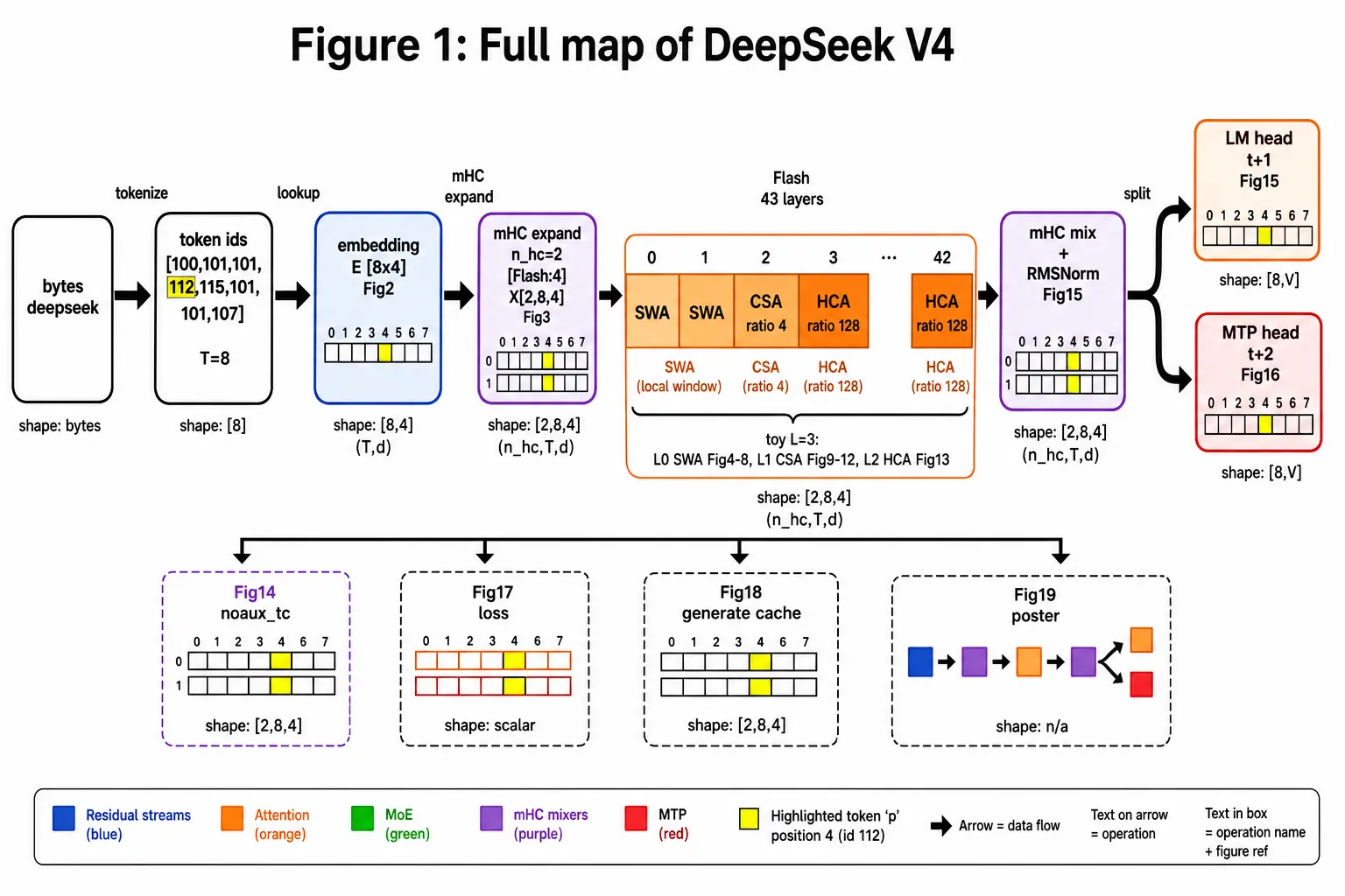
<p>Token ids, embedding, mHC expand into <code class="language-plaintext highlighter-rouge">hc_mult = 4</code> residual streams, then 43 layers of attention plus DeepSeekMoE, each wrapped by mHC, then mix, RMSNorm, a main LM head for token $t+1$, and one MTP block for $t+2$.</p>

<pre><code class="language-mermaid">flowchart TD
  ids["token ids"] --&gt; emb["embedding"]
  emb --&gt; exp["mHC expand, n_hc streams"]
  exp --&gt; blk["block x 43"]
  blk --&gt; mix["mHC mix + RMSNorm"]
  mix --&gt; lm["LM head: token t+1"]
  mix --&gt; mtp["MTP depth 1: token t+2"]
  subgraph one ["one block"]
    attn["SWA or CSA or HCA"]
    moe["DeepSeekMoE"]
    attn --&gt; moe
  end
  blk --- one
</code></pre>

<p><code class="language-plaintext highlighter-rouge">compress_ratios</code> in Flash-0731 starts <code class="language-plaintext highlighter-rouge">[0, 0, 4, 128, ...]</code>. Layers 0 and 1 are sliding-window only. After that, CSA ($m = 4$) and HCA ($m’ = 128$) alternate. The JSON lists a few trailing zeros after layer 42; <code class="language-plaintext highlighter-rouge">num_hidden_layers</code> is 43, so I am only reading the first 43 slots.</p>

<div data-title="DeepSeek-V4-Flash-0731/config.json" class="language-json highlighter-rouge"><div class="highlight"><pre class="highlight"><code><span class="p">{</span><span class="w">
  </span><span class="nl">"hidden_size"</span><span class="p">:</span><span class="w"> </span><span class="mi">4096</span><span class="p">,</span><span class="w">
  </span><span class="nl">"num_hidden_layers"</span><span class="p">:</span><span class="w"> </span><span class="mi">43</span><span class="p">,</span><span class="w">
  </span><span class="nl">"num_attention_heads"</span><span class="p">:</span><span class="w"> </span><span class="mi">64</span><span class="p">,</span><span class="w">
  </span><span class="nl">"head_dim"</span><span class="p">:</span><span class="w"> </span><span class="mi">512</span><span class="p">,</span><span class="w">
  </span><span class="nl">"num_key_value_heads"</span><span class="p">:</span><span class="w"> </span><span class="mi">1</span><span class="p">,</span><span class="w">
  </span><span class="nl">"q_lora_rank"</span><span class="p">:</span><span class="w"> </span><span class="mi">1024</span><span class="p">,</span><span class="w">
  </span><span class="nl">"qk_rope_head_dim"</span><span class="p">:</span><span class="w"> </span><span class="mi">64</span><span class="p">,</span><span class="w">
  </span><span class="nl">"index_topk"</span><span class="p">:</span><span class="w"> </span><span class="mi">512</span><span class="p">,</span><span class="w">
  </span><span class="nl">"sliding_window"</span><span class="p">:</span><span class="w"> </span><span class="mi">128</span><span class="p">,</span><span class="w">
  </span><span class="nl">"n_routed_experts"</span><span class="p">:</span><span class="w"> </span><span class="mi">256</span><span class="p">,</span><span class="w">
  </span><span class="nl">"num_experts_per_tok"</span><span class="p">:</span><span class="w"> </span><span class="mi">6</span><span class="p">,</span><span class="w">
  </span><span class="nl">"n_shared_experts"</span><span class="p">:</span><span class="w"> </span><span class="mi">1</span><span class="p">,</span><span class="w">
  </span><span class="nl">"moe_intermediate_size"</span><span class="p">:</span><span class="w"> </span><span class="mi">2048</span><span class="p">,</span><span class="w">
  </span><span class="nl">"num_hash_layers"</span><span class="p">:</span><span class="w"> </span><span class="mi">3</span><span class="p">,</span><span class="w">
  </span><span class="nl">"scoring_func"</span><span class="p">:</span><span class="w"> </span><span class="s2">"sqrtsoftplus"</span><span class="p">,</span><span class="w">
  </span><span class="nl">"topk_method"</span><span class="p">:</span><span class="w"> </span><span class="s2">"noaux_tc"</span><span class="p">,</span><span class="w">
  </span><span class="nl">"hc_mult"</span><span class="p">:</span><span class="w"> </span><span class="mi">4</span><span class="p">,</span><span class="w">
  </span><span class="nl">"hc_sinkhorn_iters"</span><span class="p">:</span><span class="w"> </span><span class="mi">20</span><span class="p">,</span><span class="w">
  </span><span class="nl">"num_nextn_predict_layers"</span><span class="p">:</span><span class="w"> </span><span class="mi">1</span><span class="p">,</span><span class="w">
  </span><span class="nl">"vocab_size"</span><span class="p">:</span><span class="w"> </span><span class="mi">129280</span><span class="p">,</span><span class="w">
  </span><span class="nl">"max_position_embeddings"</span><span class="p">:</span><span class="w"> </span><span class="mi">1048576</span><span class="p">,</span><span class="w">
  </span><span class="nl">"swiglu_limit"</span><span class="p">:</span><span class="w"> </span><span class="mf">10.0</span><span class="w">
</span><span class="p">}</span><span class="w">
</span></code></pre></div></div>

<table>
  <thead>
    <tr>
      <th>Knob</th>
      <th style="text-align: right">Toy (these figures)</th>
      <th style="text-align: right">Flash-0731</th>
      <th style="text-align: right">Pro (paper)</th>
    </tr>
  </thead>
  <tbody>
    <tr>
      <td>Total / active</td>
      <td style="text-align: right">n/a</td>
      <td style="text-align: right">284B / 13B</td>
      <td style="text-align: right">1.6T / 49B</td>
    </tr>
    <tr>
      <td>Layers</td>
      <td style="text-align: right">3</td>
      <td style="text-align: right">43</td>
      <td style="text-align: right">n/a</td>
    </tr>
    <tr>
      <td>Hidden $d$</td>
      <td style="text-align: right">4</td>
      <td style="text-align: right">4096</td>
      <td style="text-align: right">n/a</td>
    </tr>
    <tr>
      <td>Heads $\times$ head dim</td>
      <td style="text-align: right">$2 \times 4$</td>
      <td style="text-align: right">$64 \times 512$</td>
      <td style="text-align: right">n/a</td>
    </tr>
    <tr>
      <td>$q$ LoRA rank</td>
      <td style="text-align: right">n/a</td>
      <td style="text-align: right">1024</td>
      <td style="text-align: right">n/a</td>
    </tr>
    <tr>
      <td>CSA $m$</td>
      <td style="text-align: right">2</td>
      <td style="text-align: right">4</td>
      <td style="text-align: right">n/a</td>
    </tr>
    <tr>
      <td>HCA $m’$</td>
      <td style="text-align: right">4</td>
      <td style="text-align: right">128</td>
      <td style="text-align: right">n/a</td>
    </tr>
    <tr>
      <td>Indexer top-$k$</td>
      <td style="text-align: right">2</td>
      <td style="text-align: right">512</td>
      <td style="text-align: right">n/a</td>
    </tr>
    <tr>
      <td>Uncompressed window</td>
      <td style="text-align: right">2</td>
      <td style="text-align: right">128</td>
      <td style="text-align: right">n/a</td>
    </tr>
    <tr>
      <td>RoPE dims</td>
      <td style="text-align: right">last 2</td>
      <td style="text-align: right">last 64</td>
      <td style="text-align: right">n/a</td>
    </tr>
    <tr>
      <td>Routed / $k$ / shared</td>
      <td style="text-align: right">4 / 2 / 1</td>
      <td style="text-align: right">256 / 6 / 1</td>
      <td style="text-align: right">n/a</td>
    </tr>
    <tr>
      <td>Expert intermediate</td>
      <td style="text-align: right">3</td>
      <td style="text-align: right">2048</td>
      <td style="text-align: right">n/a</td>
    </tr>
    <tr>
      <td>Hash MoE layers</td>
      <td style="text-align: right">1 (layer 0)</td>
      <td style="text-align: right">3</td>
      <td style="text-align: right">n/a</td>
    </tr>
    <tr>
      <td>$n_{hc}$ / Sinkhorn iters</td>
      <td style="text-align: right">2 / 3</td>
      <td style="text-align: right">4 / 20</td>
      <td style="text-align: right">n/a</td>
    </tr>
    <tr>
      <td>MTP depth</td>
      <td style="text-align: right">1</td>
      <td style="text-align: right">1</td>
      <td style="text-align: right">1</td>
    </tr>
    <tr>
      <td>Vocab</td>
      <td style="text-align: right">256 (bytes)</td>
      <td style="text-align: right">129280</td>
      <td style="text-align: right">n/a</td>
    </tr>
    <tr>
      <td>Context</td>
      <td style="text-align: right">8</td>
      <td style="text-align: right">$1{,}048{,}576$</td>
      <td style="text-align: right">$1{,}000{,}000$</td>
    </tr>
  </tbody>
</table>

<p><img src="/assets/images/deepseek-v4-inside/fig01-full-map.webp" alt="Full map of DeepSeek V4: bytes to embedding to mHC streams to 43 hybrid-attention MoE blocks to LM head and MTP" title="Figure 1: full map. Yellow is p. Flash strip is SWA, SWA, then 4/128 alternating." /></p>

<h2 id="how-does-deepseek-become-an-8-times-4-matrix">How does “deepseek” become an $8 \times 4$ matrix?</h2>

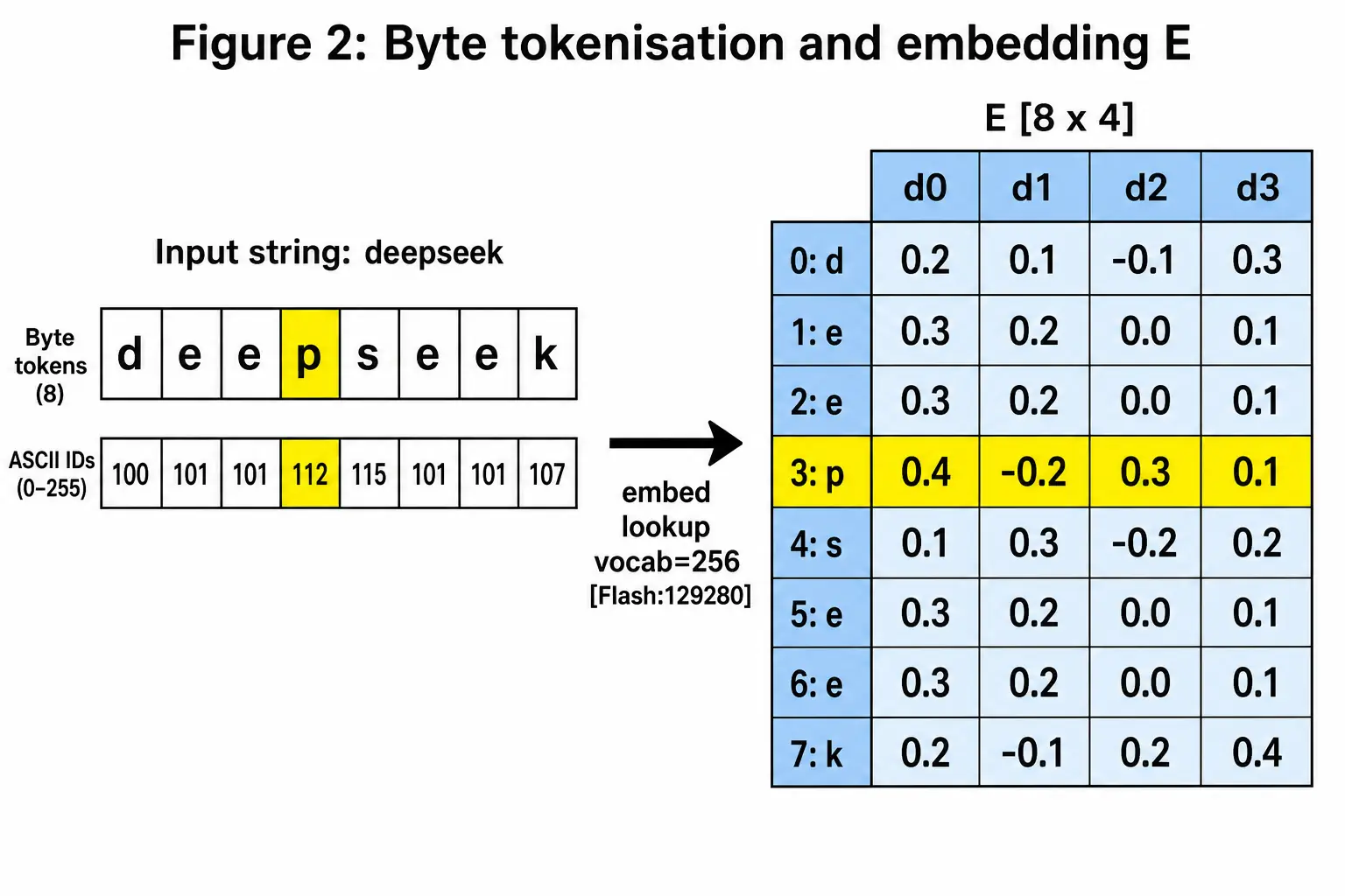
<p>Raw bytes, not BPE. Ids <code class="language-plaintext highlighter-rouge">[100, 101, 101, 112, 115, 101, 101, 107]</code>. That is <code class="language-plaintext highlighter-rouge">d e e p s e e k</code>. Yellow <strong>p</strong> is ASCII 112.</p>

<p><img src="/assets/images/deepseek-v4-inside/fig02-byte-embedding.webp" alt="Byte tokenisation of deepseek and the 8 by 4 embedding matrix with row p highlighted" title="Figure 2: embedding E, shape [8 x 4]." /></p>

<p>I chose $E$ with one decimal. Yellow row:</p>

<div class="kdmath">$$
E_p = [0.6,\ -0.3,\ 0.4,\ 0.2]
$$</div>

<p>Flash vocab is 129280. The toy vocab is 256 so the picture fits. Same gather: id $\to$ row of $E$. See <a href="/blog/token-embeddings-explained/">token embeddings</a> for the full-size version of that lookup.</p>

<h2 id="how-does-mhc-turn-one-stream-into-two">How does mHC turn one stream into two?</h2>

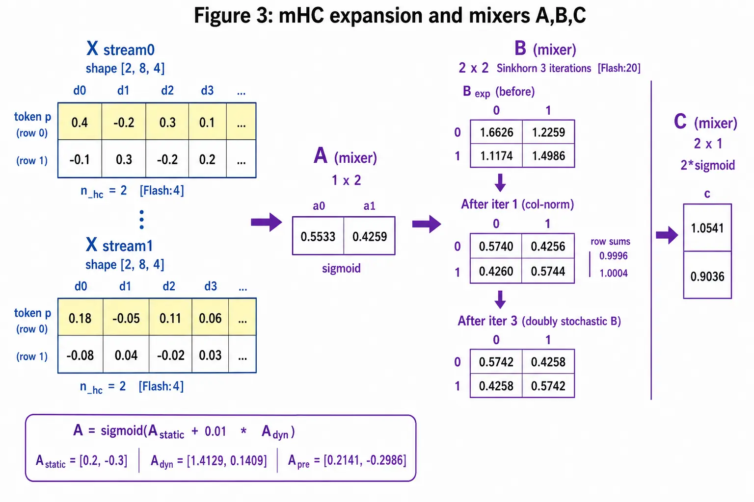
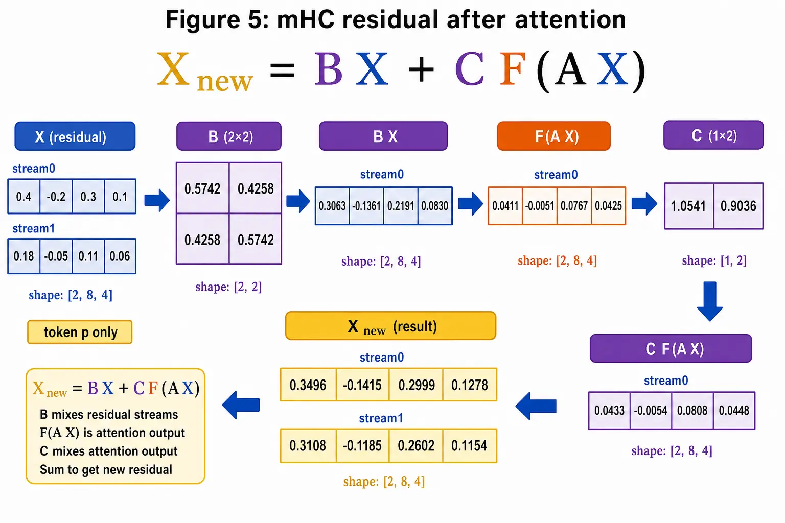
<p>Paper §2.2: the residual is $n_{hc}$ streams, not one vector of width $d$. Update</p>

<div class="kdmath">$$
X_{l+1} = B_l X_l + C_l F_l(A_l X_l)
$$</div>

<p>$A$ mixes streams into the block. $C$ writes the block output back. $B$ mixes the residual and is projected onto doubly stochastic matrices by Sinkhorn-Knopp: $M^{(0)}=\exp(\tilde B)$, then alternate row-normalize and column-normalize, Flash <code class="language-plaintext highlighter-rouge">hc_sinkhorn_iters = 20</code>. I froze $A,B,C$ after this figure so the later arithmetic stays traceable. Flash would recompute a tiny input-dependent term each time ($\alpha = 0.01$ in the toy).</p>

<p>Expand with $w = [1.0,\ 0.4]$:</p>

<table>
  <thead>
    <tr>
      <th>Stream</th>
      <th>Yellow $p$</th>
    </tr>
  </thead>
  <tbody>
    <tr>
      <td>0</td>
      <td>$[0.6,\ -0.3,\ 0.4,\ 0.2]$</td>
    </tr>
    <tr>
      <td>1</td>
      <td>$[0.24,\ -0.12,\ 0.16,\ 0.08]$</td>
    </tr>
  </tbody>
</table>

<p>Mean-pool the whole $X$ into 8 numbers, RMSNorm, then the dynamic gates. After sigmoid / $2\cdot$sigmoid:</p>

<div class="kdmath">$$
A = [0.6002,\ 0.4504],\quad C = [1.0523,\ 0.8515]
$$</div>

<p>$B$ after three Sinkhorn iterations (row sums and column sums both 1.0):</p>

<div class="kdmath">$$
B = \begin{bmatrix} 0.5741 & 0.4259 \\ 0.4259 & 0.5741 \end{bmatrix}
$$</div>

<table>
  <thead>
    <tr>
      <th>Stage</th>
      <th>$M$</th>
      <th>Row sums</th>
      <th>Col sums</th>
    </tr>
  </thead>
  <tbody>
    <tr>
      <td>$\exp(B_{\text{raw}})$</td>
      <td>$2.2381,\ 1.1101$ / $1.4957,\ 1.3482$</td>
      <td>$3.3482,\ 2.8439$</td>
      <td>$3.7338,\ 2.4583$</td>
    </tr>
    <tr>
      <td>Iter 1 row</td>
      <td>$0.6685,\ 0.3315$ / $0.5259,\ 0.4741$</td>
      <td>$1.0,\ 1.0$</td>
      <td>$1.1944,\ 0.8056$</td>
    </tr>
    <tr>
      <td>Iter 1 col</td>
      <td>$0.5597,\ 0.4115$ / $0.4403,\ 0.5885$</td>
      <td>$0.9712,\ 1.0288$</td>
      <td>$1.0,\ 1.0$</td>
    </tr>
    <tr>
      <td>Iter 3 col $= B$</td>
      <td>$0.5741,\ 0.4259$ / $0.4259,\ 0.5741$</td>
      <td>$1.0,\ 1.0$</td>
      <td>$1.0,\ 1.0$</td>
    </tr>
  </tbody>
</table>

<p><img src="/assets/images/deepseek-v4-inside/fig03-mhc-expand.webp" alt="mHC expansion of E into two residual streams and Sinkhorn iterations on mixer B" title="Figure 3: mHC expand. B ends doubly stochastic." /></p>

<p>A doubly stochastic $B$ cannot amplify the residual without bound as depth goes to 43. That is the point of the manifold constraint. The 20 iterations in Flash are cheap relative to attention at 1M tokens; they are not cheap relative to a 2×2 toy.</p>

<h2 id="what-does-layer-0-sliding-window-attention-do-to-p">What does layer 0 sliding-window attention do to p?</h2>

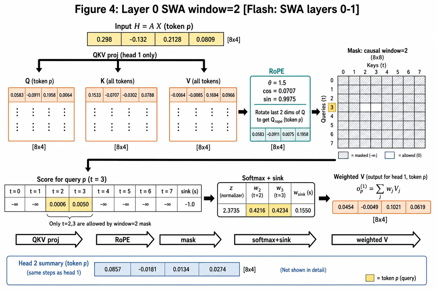
<p>Collapse streams: $H = A X$. Yellow:</p>

<div class="kdmath">$$
H_p = 0.6002\cdot[0.6,\ -0.3,\ 0.4,\ 0.2] + 0.4504\cdot[0.24,\ -0.12,\ 0.16,\ 0.08] = [0.4682,\ -0.2341,\ 0.3121,\ 0.1561]
$$</div>

<p>Head 1, after $W_Q,W_K,W_V$:</p>

<table>
  <thead>
    <tr>
      <th> </th>
      <th style="text-align: right">0</th>
      <th style="text-align: right">1</th>
      <th style="text-align: right">2</th>
      <th style="text-align: right">3</th>
    </tr>
  </thead>
  <tbody>
    <tr>
      <td>$Q$</td>
      <td style="text-align: right">0.1717</td>
      <td style="text-align: right">−0.0936</td>
      <td style="text-align: right">0.1951</td>
      <td style="text-align: right">0.1014</td>
    </tr>
    <tr>
      <td>$K$</td>
      <td style="text-align: right">0.2185</td>
      <td style="text-align: right">−0.0702</td>
      <td style="text-align: right">0.0078</td>
      <td style="text-align: right">0.2887</td>
    </tr>
    <tr>
      <td>$V$</td>
      <td style="text-align: right">0.1170</td>
      <td style="text-align: right">−0.0312</td>
      <td style="text-align: right">0.2185</td>
      <td style="text-align: right">0.0000</td>
    </tr>
  </tbody>
</table>

<p>RoPE on the last 2 dims, position $i=3$: $\cos 3 = -0.9900$, $\sin 3 = 0.1411$.</p>

<div class="kdmath">$$
\begin{aligned}
x' &= 0.1951(-0.9900) - 0.1014(0.1411) = -0.2074 \\
y' &= 0.1951(0.1411) + 0.1014(-0.9900) = -0.0729
\end{aligned}
$$</div>

<p>Window 2, causal: $p$ sees the previous <code class="language-plaintext highlighter-rouge">e</code> and itself. Scale $1/\sqrt{4}=0.5$. Sink logit $s=-1.0$ goes in the <strong>denominator</strong> only, paper eq. (27):</p>

<div class="kdmath">$$
s_{h,i,j} = \frac{\exp(z_{h,i,j})}{\sum_k \exp(z_{h,i,k}) + \exp(z'_h)}
$$</div>

<table>
  <thead>
    <tr>
      <th>Key</th>
      <th style="text-align: right">$q\cdot k$</th>
      <th style="text-align: right">Score</th>
      <th style="text-align: right">$\exp$</th>
    </tr>
  </thead>
  <tbody>
    <tr>
      <td>pos 3 (<code class="language-plaintext highlighter-rouge">e</code>)</td>
      <td style="text-align: right">−0.0025</td>
      <td style="text-align: right">−0.0012</td>
      <td style="text-align: right">0.9988</td>
    </tr>
    <tr>
      <td>pos 4 (<code class="language-plaintext highlighter-rouge">p</code>)</td>
      <td style="text-align: right">0.0749</td>
      <td style="text-align: right">0.0374</td>
      <td style="text-align: right">1.0382</td>
    </tr>
    <tr>
      <td>sink</td>
      <td style="text-align: right">n/a</td>
      <td style="text-align: right">−1.0</td>
      <td style="text-align: right">0.3679</td>
    </tr>
  </tbody>
</table>

<p>Denom $2.4048$. Weights $0.4153$ and $0.4317$. Sink mass $0.1530$. The keys do not sum to 1. That leftover is the sink: the head is allowed to attend to nothing.</p>

<div class="kdmath">$$
\text{ctx} = [0.0797,\ 0.0837,\ 0.0716,\ 0.0000]
$$</div>

<p>Head 2 is a summary row in the figure. Concat both heads, grouped $W_O$ (Flash: 64 heads in <code class="language-plaintext highlighter-rouge">o_groups = 8</code>):</p>

<div class="kdmath">$$
F_{\text{attn}} = [0.0415,\ 0.1235,\ -0.0035,\ 0.0665]
$$</div>

<p><img src="/assets/images/deepseek-v4-inside/fig04-layer0-swa.webp" alt="Layer 0 sliding-window attention for token p with RoPE, window-2 mask, and sink softmax" title="Figure 4: layer 0 SWA, window 2. Flash layers 0-1 use compress_ratio 0." /></p>

<p>Flash keeps a 128-token uncompressed window even after compression starts (<code class="language-plaintext highlighter-rouge">sliding_window</code>). The first two layers never compress. Local syntax is cheap. The 1M problem is the far tokens.</p>

<h2 id="how-does-the-residual-update-after-attention">How does the residual update after attention?</h2>

<div class="kdmath">$$
X_{\text{new}} = B X + C F
$$</div>

<p>Yellow stream 0:</p>

<div class="kdmath">$$
\begin{aligned}
BX_0 &= 0.5741\cdot[0.6,\ -0.3,\ 0.4,\ 0.2] + 0.4259\cdot[0.24,\ -0.12,\ 0.16,\ 0.08] \\
&= [0.4467,\ -0.2233,\ 0.2978,\ 0.1489] \\
C_0 F &= 1.0523\cdot F = [0.0437,\ 0.1300,\ -0.0037,\ 0.0699] \\
X_{\text{new},0} &= [0.4904,\ -0.0934,\ 0.2941,\ 0.2188]
\end{aligned}
$$</div>

<p>Stream 1 lands at $[0.4287,\ -0.0915,\ 0.2592,\ 0.1877]$.</p>

<p><img src="/assets/images/deepseek-v4-inside/fig05-mhc-after-attn.webp" alt="mHC residual update after attention: B mixes streams, C scales the attention output" title="Figure 5: X_new = B X + C F after attention." /></p>

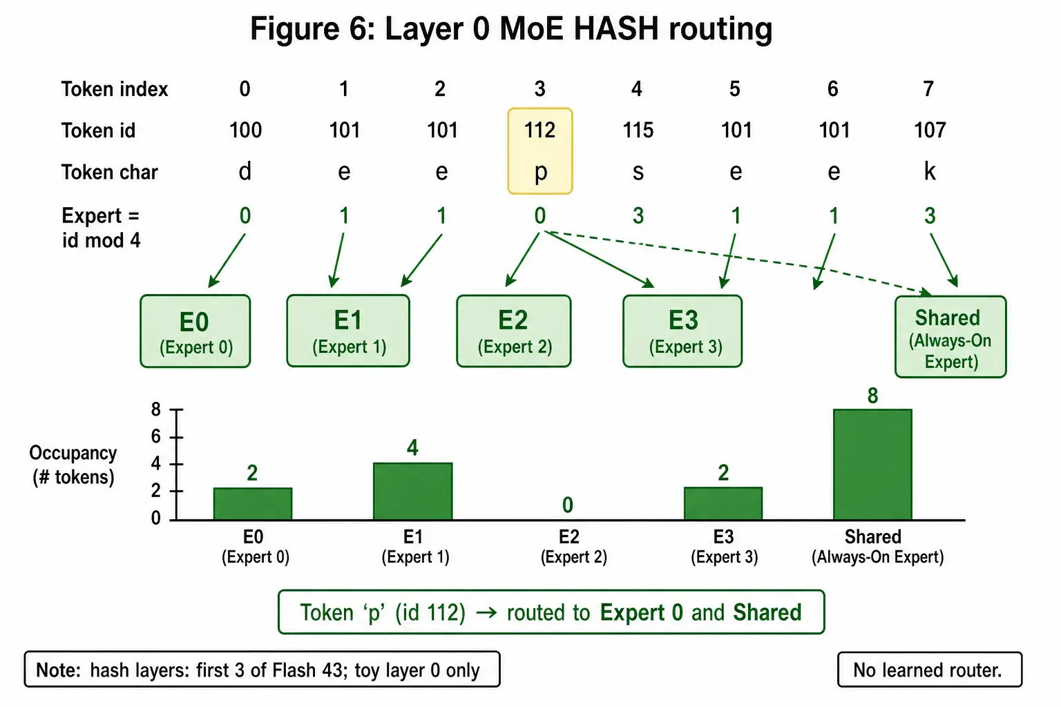
<h2 id="why-does-layer-0-moe-hash-the-token-id">Why does layer 0 MoE hash the token id?</h2>

<p>Config: <code class="language-plaintext highlighter-rouge">num_hash_layers = 3</code>. Paper §2.1: the first MoE layers replace a learned router with hash routing, expert from the token id, no dense FFN at the start the way V3 had.</p>

<p>Toy: <code class="language-plaintext highlighter-rouge">expert = token_id mod 4</code>. Second routed expert is <code class="language-plaintext highlighter-rouge">(e+1) mod 4</code> so top-2 still fires. Shared expert always on. Hash has no logits, so I fixed gates $0.7$ and $0.3$.</p>

<table>
  <thead>
    <tr>
      <th>Token</th>
      <th style="text-align: right">Id</th>
      <th style="text-align: right">Primary</th>
      <th style="text-align: right">Second</th>
    </tr>
  </thead>
  <tbody>
    <tr>
      <td>d</td>
      <td style="text-align: right">100</td>
      <td style="text-align: right">0</td>
      <td style="text-align: right">1</td>
    </tr>
    <tr>
      <td>e</td>
      <td style="text-align: right">101</td>
      <td style="text-align: right">1</td>
      <td style="text-align: right">2</td>
    </tr>
    <tr>
      <td>e</td>
      <td style="text-align: right">101</td>
      <td style="text-align: right">1</td>
      <td style="text-align: right">2</td>
    </tr>
    <tr>
      <td><strong>p</strong></td>
      <td style="text-align: right"><strong>112</strong></td>
      <td style="text-align: right"><strong>0</strong></td>
      <td style="text-align: right"><strong>1</strong></td>
    </tr>
    <tr>
      <td>s</td>
      <td style="text-align: right">115</td>
      <td style="text-align: right">3</td>
      <td style="text-align: right">0</td>
    </tr>
    <tr>
      <td>e</td>
      <td style="text-align: right">101</td>
      <td style="text-align: right">1</td>
      <td style="text-align: right">2</td>
    </tr>
    <tr>
      <td>e</td>
      <td style="text-align: right">101</td>
      <td style="text-align: right">1</td>
      <td style="text-align: right">2</td>
    </tr>
    <tr>
      <td>k</td>
      <td style="text-align: right">107</td>
      <td style="text-align: right">3</td>
      <td style="text-align: right">0</td>
    </tr>
  </tbody>
</table>

<p>Occupancy of the hashed primary: $[2,\ 4,\ 0,\ 2]$. Expert 2 is empty. That is why later layers switch to a learned router plus <code class="language-plaintext highlighter-rouge">noaux_tc</code> bias.</p>

<p><img src="/assets/images/deepseek-v4-inside/fig06-hash-routing.webp" alt="Layer 0 hash routing: token id mod 4, shared expert always on, occupancy bars" title="Figure 6: hash routing. Flash hashes the first 3 MoE layers." /></p>

<p>Input to the expert, after mixing the post-attention streams:</p>

<div class="kdmath">$$
h_p = [0.4874,\ -0.0973,\ 0.2933,\ 0.2159]
$$</div>

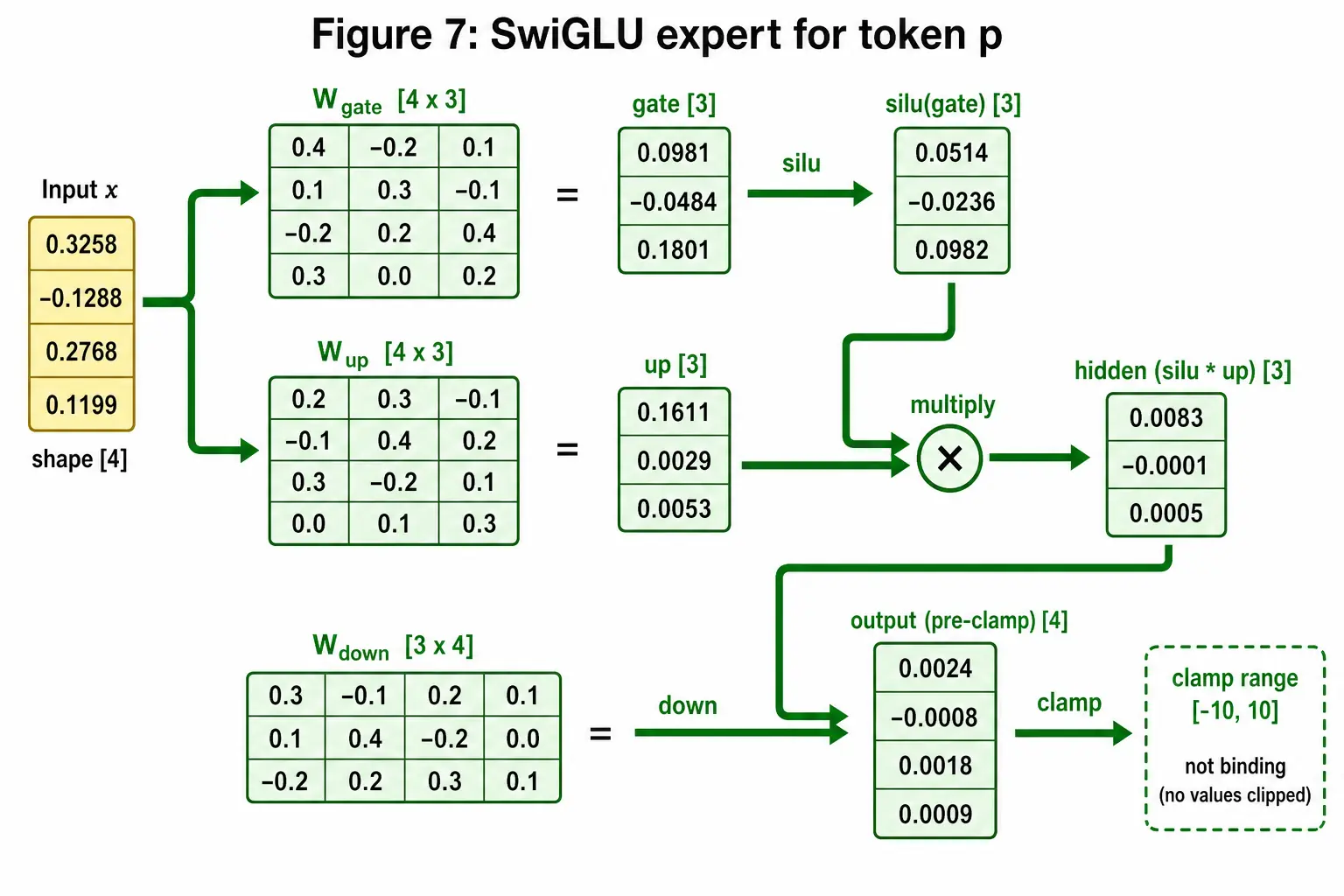
<p>Expert 0 is SwiGLU, intermediate 3 (Flash 2048), output clamped to $[-10,10]$ (<code class="language-plaintext highlighter-rouge">swiglu_limit</code>).</p>

<div class="kdmath">$$
\text{gate} = h W_{\text{gate}} = [0.2109,\ 0.0449,\ 0.0533]
$$</div>

<p>$\mathrm{SiLU}(g)=g\cdot\sigma(g)$:</p>

<table>
  <thead>
    <tr>
      <th style="text-align: right">$g$</th>
      <th style="text-align: right">$\sigma(g)$</th>
      <th style="text-align: right">SiLU</th>
      <th style="text-align: right">$\times$ up</th>
      <th style="text-align: right">hid</th>
    </tr>
  </thead>
  <tbody>
    <tr>
      <td style="text-align: right">0.2109</td>
      <td style="text-align: right">0.5525</td>
      <td style="text-align: right">0.1166</td>
      <td style="text-align: right">0.1520</td>
      <td style="text-align: right">0.0177</td>
    </tr>
    <tr>
      <td style="text-align: right">0.0449</td>
      <td style="text-align: right">0.5112</td>
      <td style="text-align: right">0.0230</td>
      <td style="text-align: right">−0.0229</td>
      <td style="text-align: right">−0.0005</td>
    </tr>
    <tr>
      <td style="text-align: right">0.0533</td>
      <td style="text-align: right">0.5133</td>
      <td style="text-align: right">0.0274</td>
      <td style="text-align: right">0.2852</td>
      <td style="text-align: right">0.0078</td>
    </tr>
  </tbody>
</table>

<p>$y = \text{hid}\,W_{\text{down}} = [0.0062,\ 0.0032,\ 0.0013,\ 0.0044]$. Clamp does not bite. On FP8/FP4 training it does; that is why the limit exists (paper §4.2.3).</p>

<p><img src="/assets/images/deepseek-v4-inside/fig07-swiglu.webp" alt="SwiGLU inside expert 0 for token p: gate, up, silu, down, clamp" title="Figure 7: one SwiGLU expert. Intermediate 3, Flash 2048." /></p>

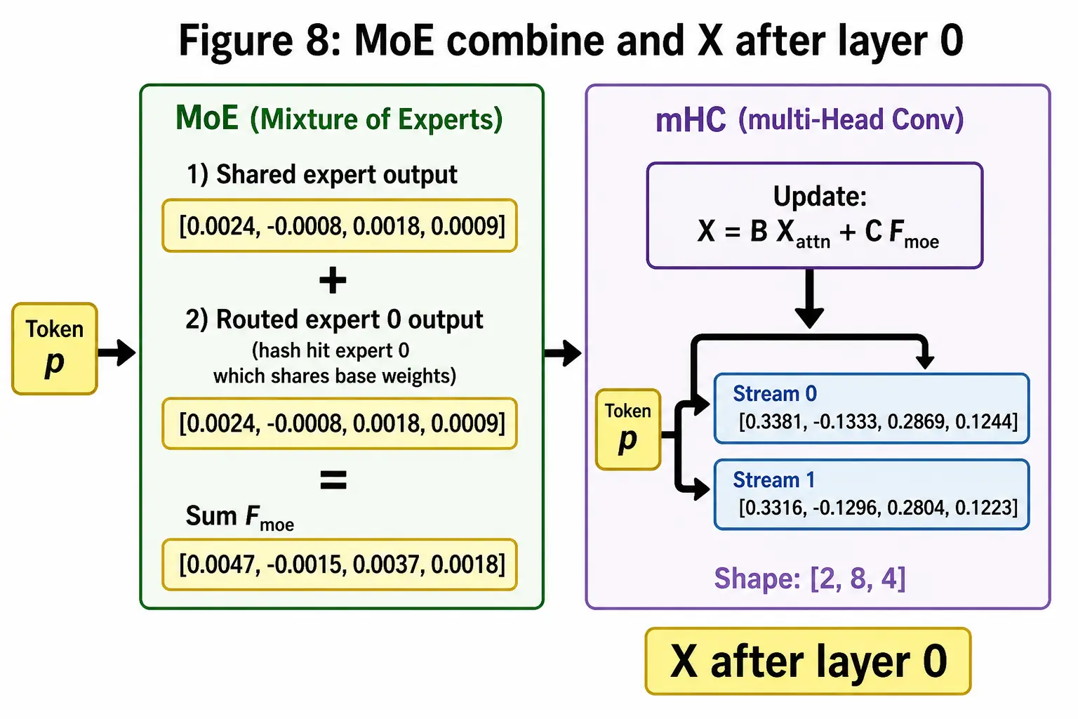
<p>Combine: shared $+$ gated routed.</p>

<table>
  <thead>
    <tr>
      <th>Path</th>
      <th>Vector</th>
    </tr>
  </thead>
  <tbody>
    <tr>
      <td>Shared</td>
      <td>$[0.0030,\ 0.0037,\ 0.0074,\ 0.0043]$</td>
    </tr>
    <tr>
      <td>Expert 0</td>
      <td>$[0.0062,\ 0.0032,\ 0.0013,\ 0.0044]$</td>
    </tr>
    <tr>
      <td>Expert 1</td>
      <td>$[0.0068,\ 0.0029,\ -0.0004,\ 0.0039]$</td>
    </tr>
    <tr>
      <td>$0.7 e_0 + 0.3 e_1$</td>
      <td>$[0.0064,\ 0.0031,\ 0.0008,\ 0.0043]$</td>
    </tr>
    <tr>
      <td>$F_{\text{MoE}}$</td>
      <td>$[0.0094,\ 0.0068,\ 0.0082,\ 0.0085]$</td>
    </tr>
  </tbody>
</table>

<p>Second mHC wrap. $X$ after layer 0, yellow:</p>

<table>
  <thead>
    <tr>
      <th>Stream</th>
      <th>$X$</th>
    </tr>
  </thead>
  <tbody>
    <tr>
      <td>0</td>
      <td>$[0.4739,\ -0.0854,\ 0.2879,\ 0.2146]$</td>
    </tr>
    <tr>
      <td>1</td>
      <td>$[0.4629,\ -0.0865,\ 0.2811,\ 0.2082]$</td>
    </tr>
  </tbody>
</table>

<p>Flash activates 6 of 256 routed experts plus 1 shared. That is the 13B-active number sitting inside 284B total.</p>

<p><img src="/assets/images/deepseek-v4-inside/fig08-moe-combine.webp" alt="MoE combine of shared and two routed experts, then mHC, X after layer 0" title="Figure 8: MoE combine and X after layer 0." /></p>

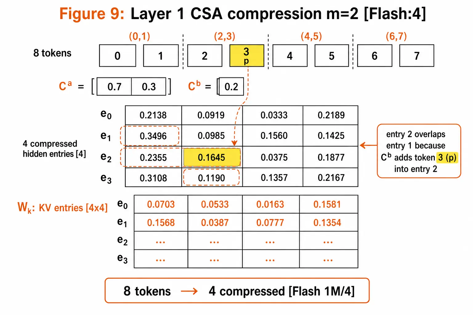
<h2 id="how-does-csa-compress-8-tokens-into-4-kv-entries">How does CSA compress 8 tokens into 4 KV entries?</h2>

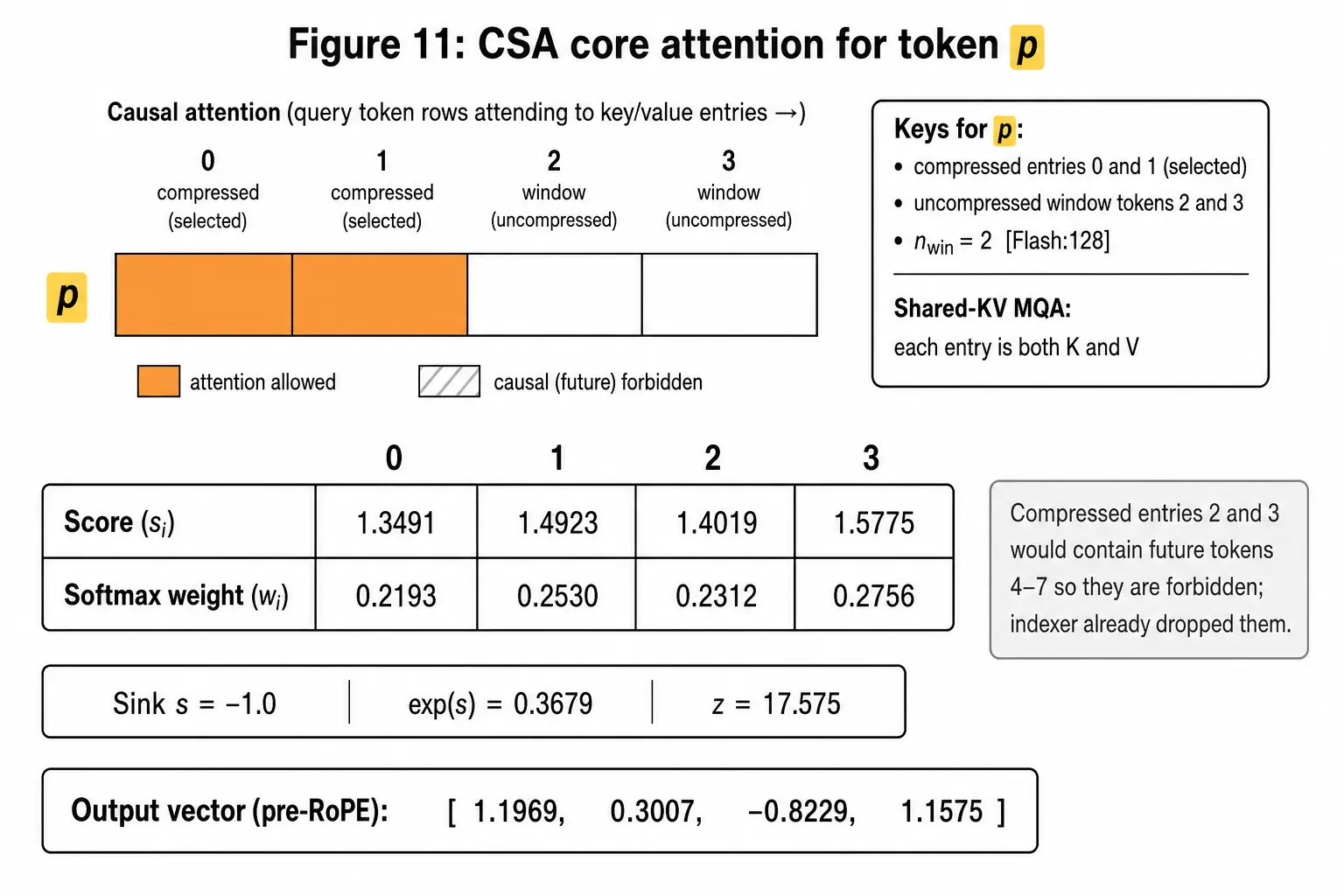
<p>Paper §2.3.1: every $m$ tokens become one KV entry by an overlapped weighted sum of two streams $C^a$ and $C^b$. Adjacent blocks share tokens. Then a lightning indexer keeps top-$k$ (Flash 512). Core attention is shared-KV MQA: the compressed entry is both $K$ and $V$. An uncompressed window of <code class="language-plaintext highlighter-rouge">sliding_window</code> tokens is concatenated so a query can see inside its own compression block without breaking causality.</p>

<p>Toy $m=2$, overlap weights $C^a=[0.5,\ 0.3]$, $C^b=[0.2]$ on the next token. Entry 2 uses tokens of entry 1. $H$ after mixing layer-0 $X$, yellow $[0.4930,\ -0.0902,\ 0.2994,\ 0.2226]$.</p>

<table>
  <thead>
    <tr>
      <th>Entry</th>
      <th>Token indices</th>
      <th>Compressed KV</th>
    </tr>
  </thead>
  <tbody>
    <tr>
      <td>0</td>
      <td>0, 1, 2</td>
      <td>$[0.3717,\ 0.3422,\ -0.0321,\ 0.0540]$</td>
    </tr>
    <tr>
      <td>1</td>
      <td>2, 3, 4</td>
      <td>$[0.2972,\ 0.2917,\ 0.1721,\ 0.0681]$</td>
    </tr>
    <tr>
      <td>2</td>
      <td>4, 5, 6</td>
      <td>$[0.1243,\ 0.4243,\ 0.1979,\ 0.1469]$</td>
    </tr>
    <tr>
      <td>3</td>
      <td>6, 7</td>
      <td>$[0.1889,\ 0.1770,\ 0.1481,\ -0.0288]$</td>
    </tr>
  </tbody>
</table>

<p>Entry 1 contains future token <code class="language-plaintext highlighter-rouge">s</code> (position 5) relative to query $p$. Causal rule: an entry is visible only if every token in it has position $\le$ the query. Entry 1 is forbidden. The indexer can still score it. Core attention must not.</p>

<p><img src="/assets/images/deepseek-v4-inside/fig09-csa-compression.webp" alt="CSA compression: 8 tokens, m=2, overlap weights Ca and Cb, four compressed KV entries" title="Figure 9: CSA compression. Entry 2 overlaps entry 1's tokens." /></p>

<blockquote>
  <p>[!GOTCHA]
Flash CSA softmax-normalizes $2m$ overlap weights per block and uses learned $C^a$, $C^b$ plus positional biases. The toy keeps three weights that sum to 1 so the grid stays countable. Same idea, not the same tensor.</p>
</blockquote>

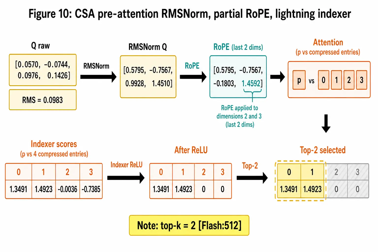
<p>RMSNorm on the Q head and on the compressed KV head, then partial RoPE on the last 2 dims (Flash last 64). Indexer scores of $p$ against the four entries, ReLU, rank:</p>

<table>
  <thead>
    <tr>
      <th>Entry</th>
      <th style="text-align: right">Score</th>
      <th style="text-align: right">ReLU</th>
      <th>Causal?</th>
    </tr>
  </thead>
  <tbody>
    <tr>
      <td>0</td>
      <td style="text-align: right">0.0891</td>
      <td style="text-align: right">0.0891</td>
      <td>yes</td>
    </tr>
    <tr>
      <td>1</td>
      <td style="text-align: right">0.1076</td>
      <td style="text-align: right">0.1076</td>
      <td><strong>no</strong> (contains <code class="language-plaintext highlighter-rouge">s</code>)</td>
    </tr>
    <tr>
      <td>2</td>
      <td style="text-align: right">0.0923</td>
      <td style="text-align: right">0.0923</td>
      <td>no</td>
    </tr>
    <tr>
      <td>3</td>
      <td style="text-align: right">0.0775</td>
      <td style="text-align: right">0.0775</td>
      <td>no</td>
    </tr>
  </tbody>
</table>

<p>Top-2 by score would be 1 then 2. After the mask, only entry 0 remains. Window $n_{\text{win}}=2$ adds uncompressed tokens 3 and 4 (<code class="language-plaintext highlighter-rouge">e</code> and <code class="language-plaintext highlighter-rouge">p</code>). Keys for core attention: 1 compressed + 2 window.</p>

<p><img src="/assets/images/deepseek-v4-inside/fig10-csa-indexer.webp" alt="CSA pre-attention: RMSNorm, partial RoPE, lightning indexer scores, ReLU, top-2, causal mask" title="Figure 10: indexer. Flash top-512. Toy top-2, then causality drops the future block." /></p>

<p><img src="/assets/images/deepseek-v4-inside/fig11-csa-core.webp" alt="CSA core attention for token p: selected compressed entry plus uncompressed window, MQA, sink, softmax" title="Figure 11: CSA core attention. Same entry is K and V." /></p>

<p>Scores for $p$, sink in the denom: $[0.9980,\ 0.1329,\ 1.9828]$, weights $[0.2362,\ 0.0994,\ 0.6323]$, sink mass $0.032$. Context $[1.4511,\ 0.2906,\ -0.6491,\ -0.3722]$.</p>

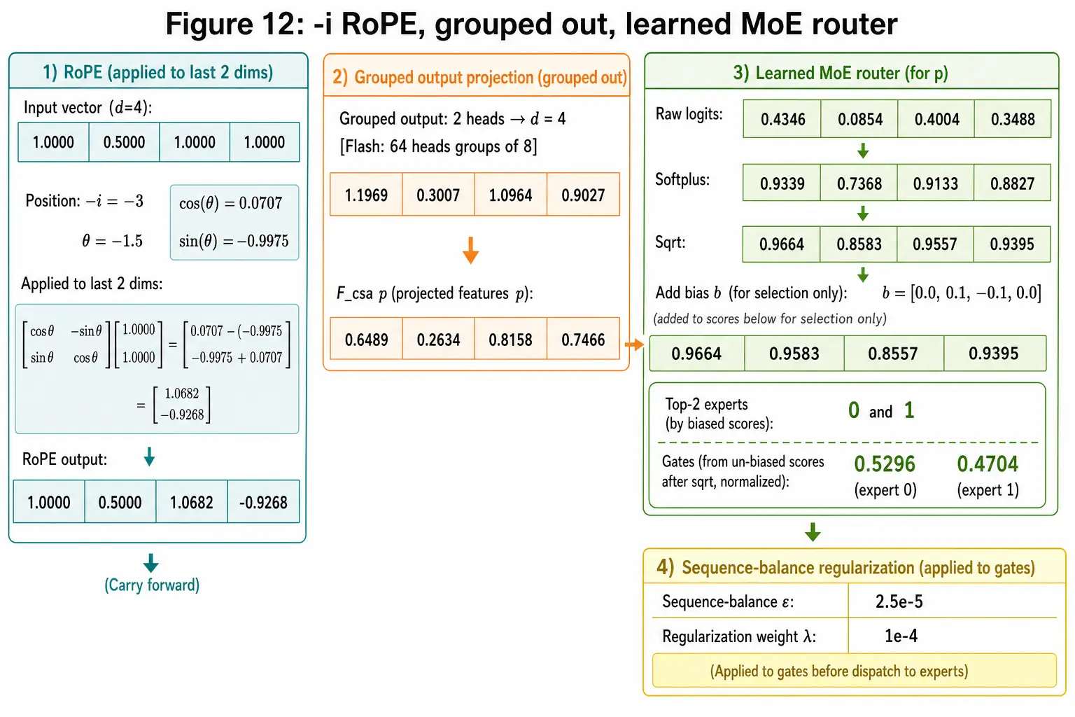
<p>Then RoPE with position $-i$ on the last 2 dims of that output. Paper: the compressed KV already carries absolute positions, so the weighted sum would leak them unless you rotate the output by $-i$. After that, grouped $W_O$:</p>

<div class="kdmath">$$
F_{\text{CSA}} = [0.8717,\ 0.9787,\ 0.0663,\ 0.6627]
$$</div>

<p>Learned router on the post-CSA hidden. Affinity is $\sqrt{\mathrm{softplus}(x)}$, not V3’s sigmoid (<code class="language-plaintext highlighter-rouge">scoring_func": "sqrtsoftplus"</code>). Bias $b=[0.0,\ 0.1,\ -0.1,\ 0.0]$ is added <strong>only</strong> for top-k selection (<code class="language-plaintext highlighter-rouge">topk_method": "noaux_tc"</code>). Gates are renormalized from the unbiased scores.</p>

<table>
  <thead>
    <tr>
      <th>Expert</th>
      <th style="text-align: right">Logit</th>
      <th style="text-align: right">softplus</th>
      <th style="text-align: right">$\sqrt{\cdot}$</th>
      <th style="text-align: right">$+$ bias</th>
      <th>Selected</th>
    </tr>
  </thead>
  <tbody>
    <tr>
      <td>0</td>
      <td style="text-align: right">0.6466</td>
      <td style="text-align: right">1.0679</td>
      <td style="text-align: right">1.0334</td>
      <td style="text-align: right">1.0334</td>
      <td>yes</td>
    </tr>
    <tr>
      <td>1</td>
      <td style="text-align: right">0.0176</td>
      <td style="text-align: right">0.7020</td>
      <td style="text-align: right">0.8378</td>
      <td style="text-align: right">0.9378</td>
      <td>no</td>
    </tr>
    <tr>
      <td>2</td>
      <td style="text-align: right">0.3729</td>
      <td style="text-align: right">0.8969</td>
      <td style="text-align: right">0.9470</td>
      <td style="text-align: right">0.8470</td>
      <td>no</td>
    </tr>
    <tr>
      <td>3</td>
      <td style="text-align: right">1.0715</td>
      <td style="text-align: right">1.3661</td>
      <td style="text-align: right">1.1688</td>
      <td style="text-align: right">1.1688</td>
      <td>yes</td>
    </tr>
  </tbody>
</table>

<p>Top-2: experts 3 and 0. Gates $0.5307$ and $0.4693$.</p>

<p><img src="/assets/images/deepseek-v4-inside/fig12-rope-router.webp" alt="Output RoPE with position minus i, grouped projection, then learned sqrt-softplus router with selection bias" title="Figure 12: output RoPE at -i, then learned router. Bias is for selection only." /></p>

<h2 id="what-does-hca-change">What does HCA change?</h2>

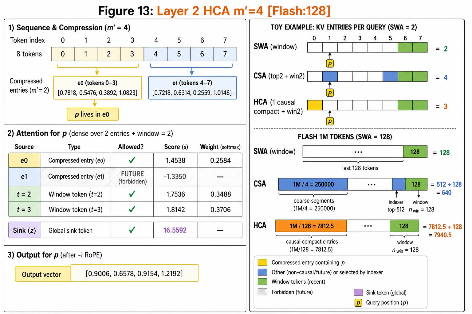
<p>Same MQA, window, RoPE, sink. Compression $m’=4$ (Flash 128), <strong>no overlap</strong>, <strong>no indexer</strong>. Dense attention over $n/m’$ entries. At toy $T=8$ that is 2 entries: tokens 0-3 and 4-7. Yellow $p$ lives in entry 0. Entry 1 still contains the future, so a causal query at $p$ only sees entry 0 plus the 2-token window.</p>

<p><img src="/assets/images/deepseek-v4-inside/fig13-hca-memory.webp" alt="HCA compression m-prime=4, dense attention over two entries plus window, KV memory bars at toy and Flash scale" title="Figure 13: HCA. No indexer. Memory bars: SWA vs CSA vs HCA." /></p>

<p>KV <strong>entries per query</strong> at Flash context $1{,}048{,}576$:</p>

<table>
  <thead>
    <tr>
      <th>Attention</th>
      <th style="text-align: right">Entries the query scores</th>
      <th>How</th>
    </tr>
  </thead>
  <tbody>
    <tr>
      <td>SWA</td>
      <td style="text-align: right">128</td>
      <td><code class="language-plaintext highlighter-rouge">sliding_window</code></td>
    </tr>
    <tr>
      <td>CSA</td>
      <td style="text-align: right">$512 + 128 = 640$</td>
      <td>indexer top-$k$ + window</td>
    </tr>
    <tr>
      <td>HCA</td>
      <td style="text-align: right">$8192 + 128 = 8320$</td>
      <td>$1{,}048{,}576/128$ dense compressed + window</td>
    </tr>
    <tr>
      <td>Plain dense</td>
      <td style="text-align: right">$1{,}048{,}576$</td>
      <td>every past token</td>
    </tr>
  </tbody>
</table>

<p>CSA is the sparse one. HCA is the heavy shrink with no indexer. Interleaving them is the hybrid in <code class="language-plaintext highlighter-rouge">compress_ratios</code>. Paper §2.3.4: mixed BF16 on the RoPE dims and FP8 on the rest, FP4 in the indexer, and versus a BF16 GQA-8 head-dim-128 baseline the 1M KV cache is about 2%. Versus DeepSeek-V3.2, Pro at 1M is 27% of the single-token FLOPs and 10% of the KV; Flash is 10% of the FLOPs and 7% of the KV.</p>

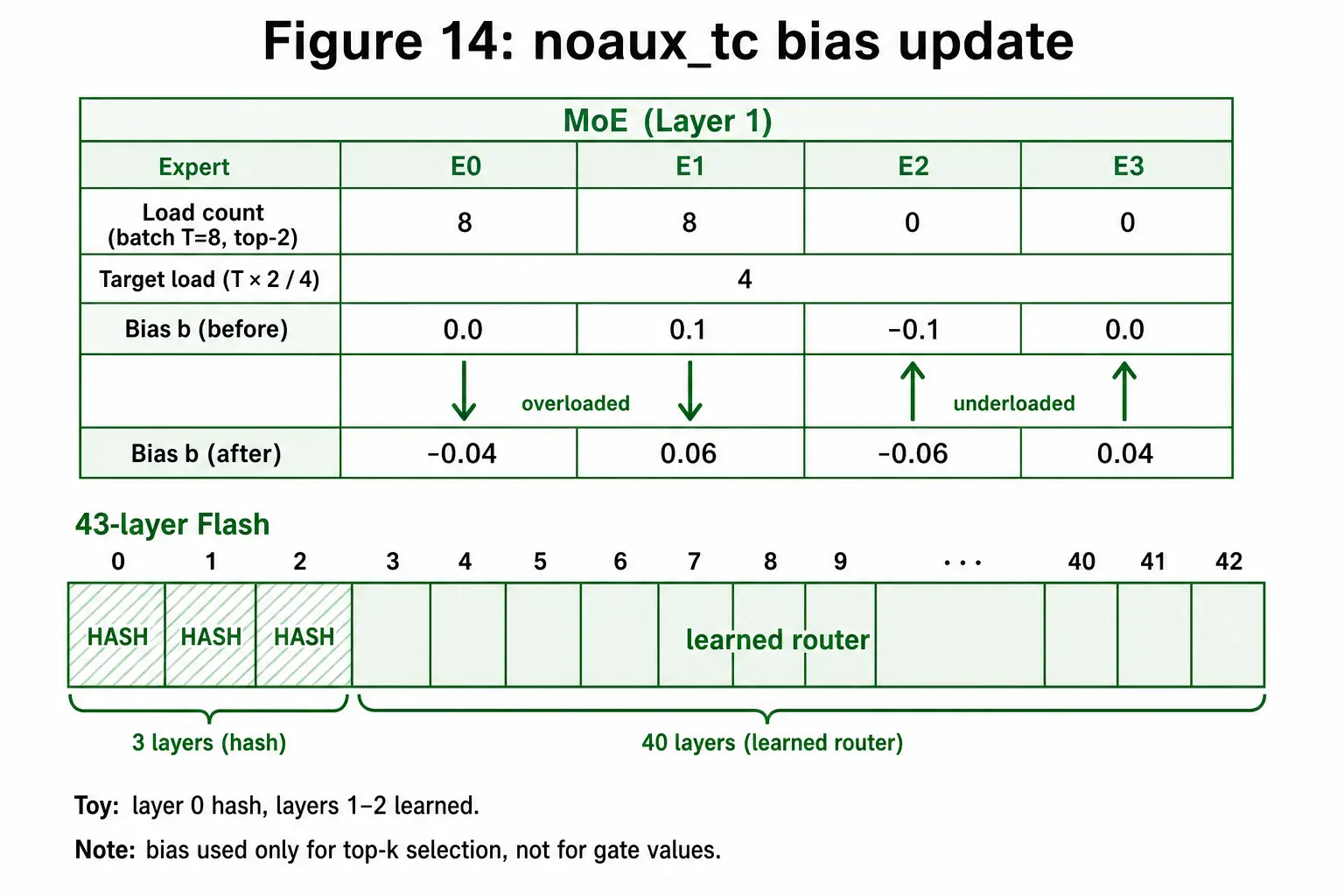
<h2 id="how-does-noaux_tc-move-expert-bias">How does noaux_tc move expert bias?</h2>

<p>No auxiliary load-balancing loss. After a batch, if expert $i$ ran hot, nudge $b_i$ down so the next batch is less likely to pick it. If it ran cold, nudge $b_i$ up. The bias does not enter the gate values, only the top-k pick. A small sequence-wise balance term stops one sequence from dumping everything on one expert (paper §2.1). Hash layers do not learn this; layers 0-2 in Flash skip the router.</p>

<p><img src="/assets/images/deepseek-v4-inside/fig14-noaux-tc.webp" alt="noaux_tc bias update from expert load counts, hash layers versus learned layers on the 43-layer strip" title="Figure 14: noaux_tc. Overloaded experts get bias down." /></p>

<p>On the toy hash layer, occupancy $[2,4,0,2]$ already shows the failure mode a learned bias is meant to fix: one expert empty, one stuffed with every <code class="language-plaintext highlighter-rouge">e</code>.</p>

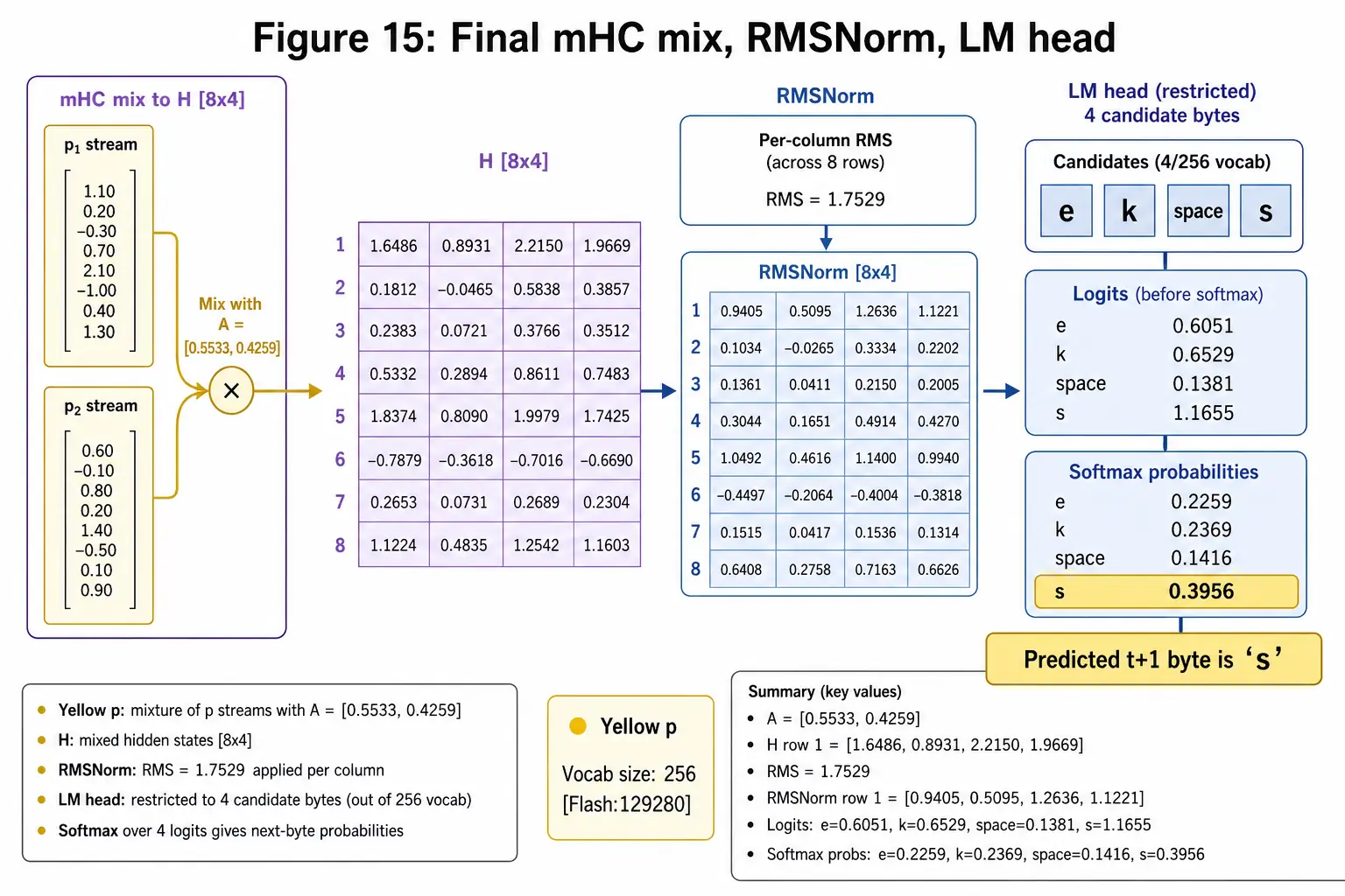
<h2 id="what-does-the-main-head-predict-for-t1">What does the main head predict for t+1?</h2>

<p>Final mix of the two streams into $[8\times 4]$, RMSNorm, LM head. Vocab 256 in the toy; I only score four candidate bytes: <code class="language-plaintext highlighter-rouge">e</code> (101), <code class="language-plaintext highlighter-rouge">k</code> (107), space (32), <code class="language-plaintext highlighter-rouge">s</code> (115). True next byte after $p$ is <code class="language-plaintext highlighter-rouge">s</code>.</p>

<p><img src="/assets/images/deepseek-v4-inside/fig15-lm-head.webp" alt="Final mHC mix, RMSNorm, LM head logits restricted to four candidate bytes, softmax for token p" title="Figure 15: main head, token t+1. Inference uses this head only." /></p>

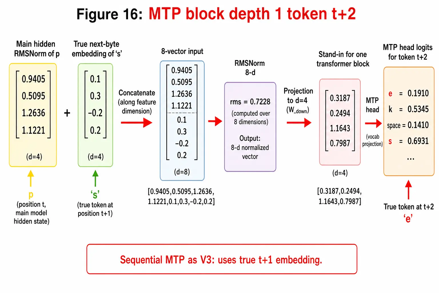
<h2 id="where-does-the-extra-t2-head-get-its-input">Where does the extra t+2 head get its input?</h2>

<p>MTP depth 1, same wiring as V3 (paper §2.1: “without modification”). During training, concatenate the main hidden state of $p$ with the embedding of the <strong>true</strong> next byte <code class="language-plaintext highlighter-rouge">s</code>, RMSNorm, a small projection, one transformer block, a second head. Inference discards this path.</p>

<p><img src="/assets/images/deepseek-v4-inside/fig16-mtp.webp" alt="MTP block: main hidden of p concatenated with embedding of true next byte, one block, logits for t+2" title="Figure 16: sequential MTP. True t+1 embedding is teacher-forced." /></p>

<h2 id="what-is-the-loss-and-who-updates-which-weights">What is the loss, and who updates which weights?</h2>

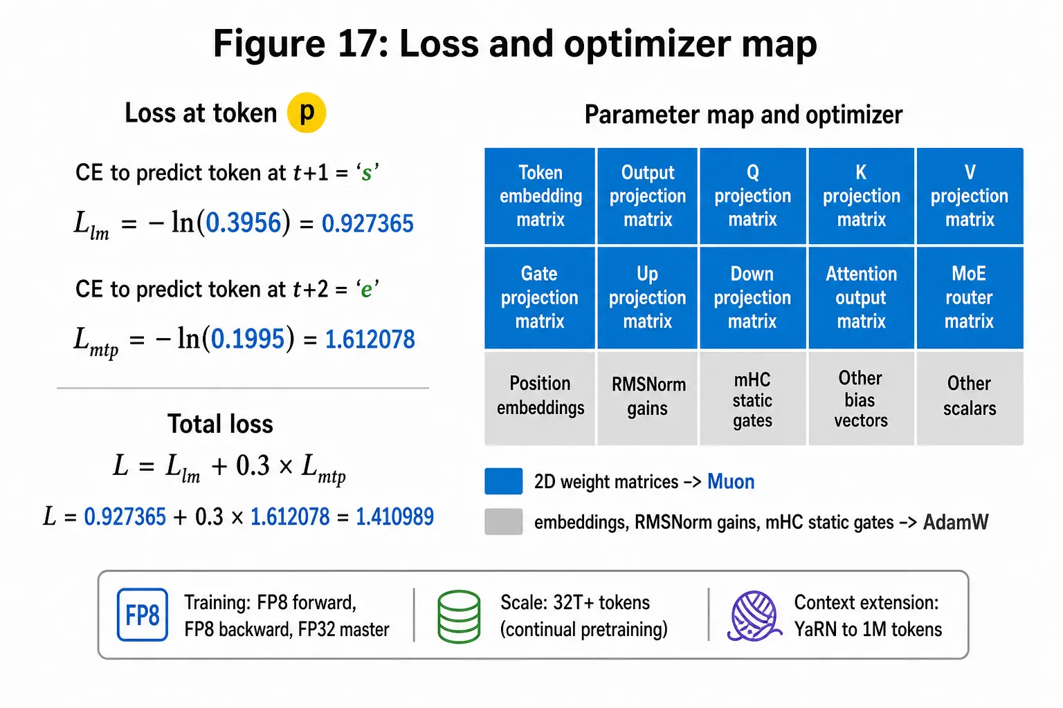
<p>V3 used $L = L_{\text{lm}} + 0.3\, L_{\text{mtp}}$. V4 keeps that MTP setup. $L_{\text{lm}}$ is cross entropy on $t+1$ (<code class="language-plaintext highlighter-rouge">s</code> for this $p$). $L_{\text{mtp}}$ is cross entropy on $t+2$ (<code class="language-plaintext highlighter-rouge">e</code>). See <a href="/blog/cross-entropy-loss-explained/">cross entropy</a> if the softmax-NLL step is rusty.</p>

<p>Muon (paper Algorithm 1, §2.4) updates the 2D weight matrices: Newton-Schulz orthogonalization of the momentum, then a scaled step. Embeddings, RMSNorm gains, and mHC static gates stay on AdamW. Training is FP8/FP4 on clusters, $32$T+ tokens, then YaRN from 64K <code class="language-plaintext highlighter-rouge">original_max_position_embeddings</code> to $1{,}048{,}576$ (<code class="language-plaintext highlighter-rouge">rope_scaling.type = yarn</code>, factor 16).</p>

<p><img src="/assets/images/deepseek-v4-inside/fig17-loss-optimizers.webp" alt="Loss L_lm plus 0.3 L_mtp at token p, and a coloured map of Muon versus AdamW parameters" title="Figure 17: MTP-weighted loss and optimizer split. Muon on 2D weights." /></p>

<h2 id="what-is-stored-at-generate-time">What is stored at generate time?</h2>

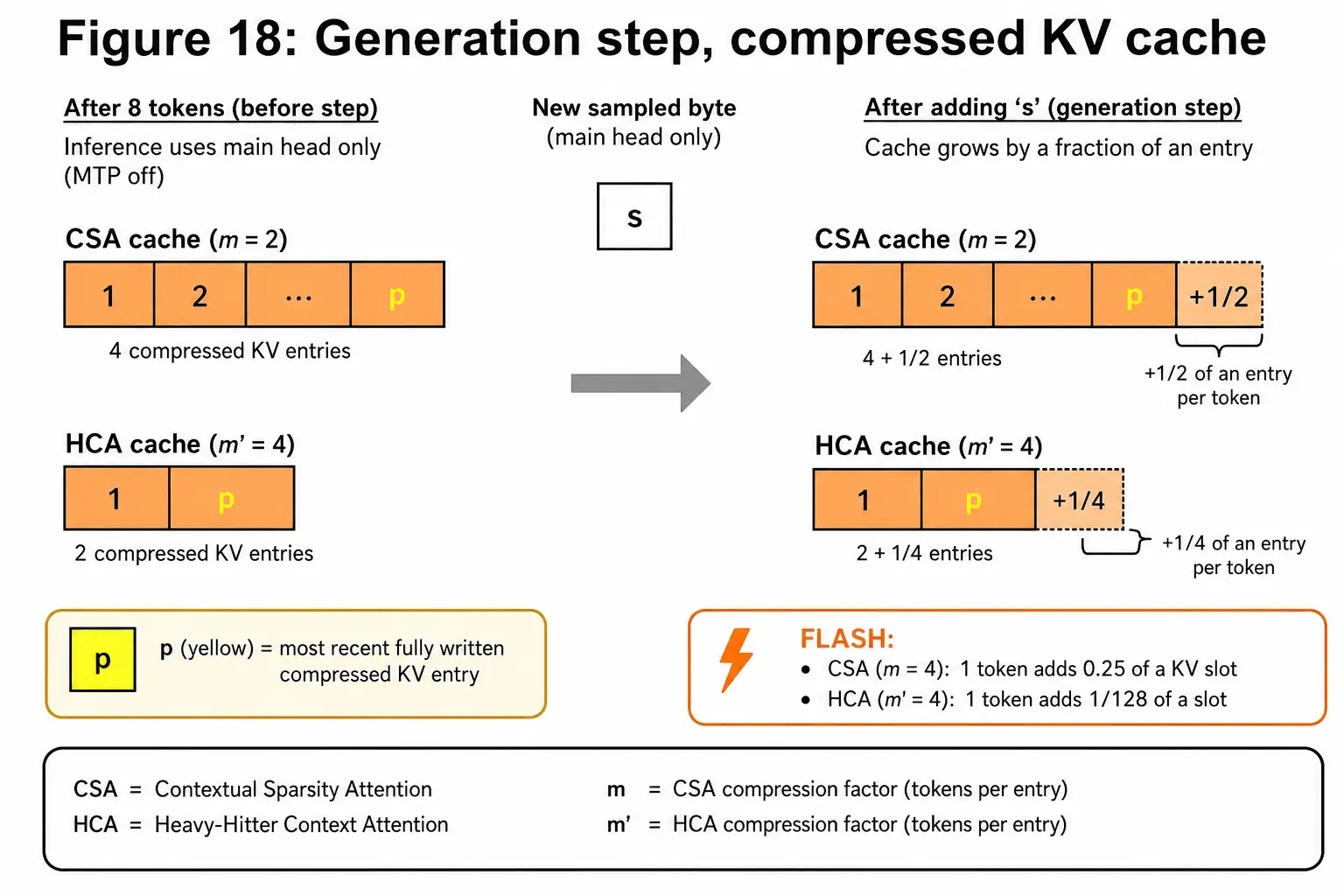
<p>Main head only. The KV cache is compressed entries, not per-token $K,V$ for every layer. After 8 toy tokens: 4 CSA entries, 2 HCA entries. The next byte grows the cache by a fraction of an entry ($1/m$ or $1/m’$), not by a full head-dim vector per layer the way a vanilla transformer does. Flash also keeps the 128-token uncompressed window.</p>

<p><img src="/assets/images/deepseek-v4-inside/fig18-generate-cache.webp" alt="Generation step: main head sample, CSA and HCA compressed KV cache after 8 tokens, cache growing by a fraction of an entry" title="Figure 18: generate. Cache is compressed entries plus a short window." /></p>

<p>That is the 1M trick in one picture: you are not storing a million keys per head. You are storing $n/4$ or $n/128$ mixed slots, plus 128 locals, plus (for CSA) a top-512 gather.</p>

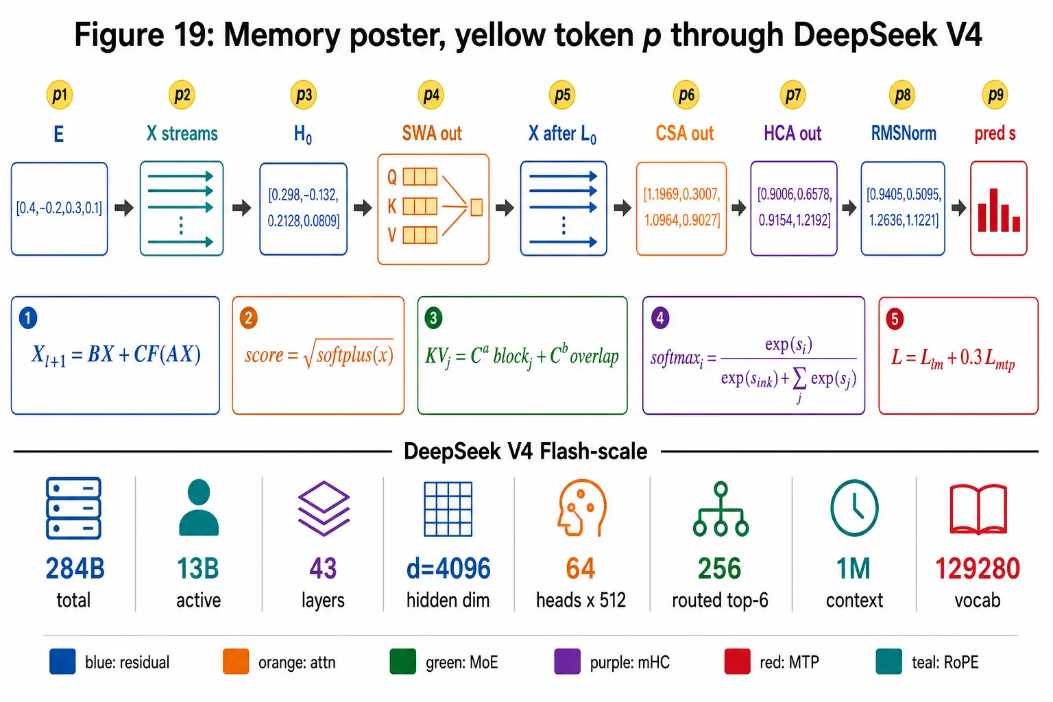
<h2 id="can-i-see-ps-numbers-on-one-page">Can I see p’s numbers on one page?</h2>

<p><img src="/assets/images/deepseek-v4-inside/fig19-memory-poster.webp" alt="One-page memory poster of the pipeline with yellow-token values, five core equations, and Flash-scale numbers" title="Figure 19: one-page poster. Five equations and the Flash knobs that matter." /></p>

<p>Five equations I actually used:</p>

<div class="kdmath">$$
\begin{aligned}
X_{l+1} &= B_l X_l + C_l F_l(A_l X_l) \\
\text{affinity} &= \sqrt{\mathrm{softplus}(x)} \\
C^{\text{Comp}}_i &= \text{overlapped weighted sum of block }i \\
s_{ij} &= \frac{\exp(z_{ij})}{\sum_k\exp(z_{ik})+\exp(z')} \\
L &= L_{\text{lm}} + \lambda L_{\text{mtp}}
\end{aligned}
$$</div>

<p>Eight Flash numbers worth keeping: 43 layers, $d=4096$, $m=4$, $m’=128$, indexer 512, window 128, 256 routed / top-6 / 1 shared, context $1{,}048{,}576$.</p>

<details>
  <summary>Shapes I would check first if I implemented the toy (batch 1, T = 8)</summary>

  <ol>
    <li>Token ids <code class="language-plaintext highlighter-rouge">[8]</code>, embedding <code class="language-plaintext highlighter-rouge">[8, 4]</code>.</li>
    <li>Residual $X$ <code class="language-plaintext highlighter-rouge">[2, 8, 4]</code>.</li>
    <li>$A X$ <code class="language-plaintext highlighter-rouge">[8, 4]</code>.</li>
    <li>Per-head $Q$ <code class="language-plaintext highlighter-rouge">[8, 4]</code>; CSA/HCA compressed KV <code class="language-plaintext highlighter-rouge">[T/m, 4]</code> or <code class="language-plaintext highlighter-rouge">[T/m', 4]</code>.</li>
    <li>SWA scores <code class="language-plaintext highlighter-rouge">[8, window]</code> with window 2.</li>
    <li>CSA indexer scores <code class="language-plaintext highlighter-rouge">[8, 4]</code> then a top-2 index tensor.</li>
    <li>MoE gates <code class="language-plaintext highlighter-rouge">[8, 2]</code> plus a shared output <code class="language-plaintext highlighter-rouge">[8, 4]</code>.</li>
    <li>Expert hidden <code class="language-plaintext highlighter-rouge">[8, 3]</code> inside SwiGLU.</li>
    <li>LM logits toy <code class="language-plaintext highlighter-rouge">[8, 256]</code>; MTP hidden concat <code class="language-plaintext highlighter-rouge">[8, 8]</code> before the projection back to 4.</li>
    <li>Cache after 8 tokens: CSA length 4, HCA length 2, window 2.</li>
  </ol>

</details>

<p><strong>Read next:</strong> the <a href="/blog/deepseek-v4-engineering-explained/">June V4 engineering notes</a> for the verification checklist and the $n^2$ cost, then <a href="/blog/attention-in-transformers-explained/">how attention works</a> if the score-row still feels like a vibe. The paper HTML is <a href="https://arxiv.org/html/2606.19348">arXiv 2606.19348</a>. The file I counted is <a href="https://huggingface.co/deepseek-ai/DeepSeek-V4-Flash-0731/blob/main/config.json">Flash-0731 <code class="language-plaintext highlighter-rouge">config.json</code></a>.</p>

<div class="footnotes" role="doc-endnotes">
  <ol>
    <li id="fn:paper">
      <p>DeepSeek-AI, <em>DeepSeek-V4: Towards Highly Efficient Million-Token Context Intelligence</em>, arXiv <a href="https://arxiv.org/abs/2606.19348">2606.19348</a>. Citation date 26 April 2026. Hybrid CSA/HCA §2.3, mHC §2.2, MoE and hash layers §2.1, MTP same as V3 §2.1, Muon §2.4, Flash/Pro widths in the abstract and §4.2.1. Checkpoints: <a href="https://huggingface.co/collections/deepseek-ai/deepseek-v4">deepseek-ai/deepseek-v4</a>. <a href="#fnref:paper" class="reversefootnote" role="doc-backlink">&#8617;</a></p>
    </li>
  </ol>
</div>]]></content><author><name>Gruhesh Sri Sai Karthik Kurra</name><email>gruheshkurra2@gmail.com</email></author><category term="ai" /><category term="DeepSeek" /><category term="LLM" /><category term="Attention" /><category term="Long Context" /><category term="Sparse Attention" /><category term="Transformers" /><category term="RoPE" /><category term="SwiGLU" /><category term="Model Training" /><summary type="html"><![CDATA[How does DeepSeek V4 process one token? I follow the byte p in deepseek through CSA, HCA, mHC, MoE, and MTP on a toy width, with Flash-0731 sizes.]]></summary><media:thumbnail xmlns:media="http://search.yahoo.com/mrss/" url="https://blogs.gruheshkurra.com/assets/images/og-deepseek-v4-inside-one-token.png" /><media:content medium="image" url="https://blogs.gruheshkurra.com/assets/images/og-deepseek-v4-inside-one-token.png" xmlns:media="http://search.yahoo.com/mrss/" /></entry><entry><title type="html">Looped Transformers Explained: Recurrent Depth and Astra</title><link href="https://blogs.gruheshkurra.com/blog/looped-transformers-explained/" rel="alternate" type="text/html" title="Looped Transformers Explained: Recurrent Depth and Astra" /><published>2026-09-03T07:30:00+00:00</published><updated>2026-09-03T07:30:00+00:00</updated><id>https://blogs.gruheshkurra.com/blog/looped-transformers-explained</id><content type="html" xml:base="https://blogs.gruheshkurra.com/blog/looped-transformers-explained/"><![CDATA[<p>I sat down with <a href="https://www.youtube.com/watch?v=KT4n-z_4QJU">Sebastian Raschka’s Astra video</a> because the rumor was doing two jobs at once: naming an architecture, and claiming that architecture hides chain of thought. The first job is checkable. The second is a jump.</p>

<p>OpenAI’s own <a href="https://openai.com/index/path-to-astra">Path to Astra</a> post (1 September 2026) confirms Astra as an upcoming model and says it meets the Critical cybersecurity threshold under their Preparedness Framework. Separate OpenAI notes on <a href="https://openai.com/index/responding-next-frontier-critical-cyber-capabilities">cyber-critical safeguards</a> describe monitors that read the model’s chain of thought and can interrupt high-risk activity. What none of those posts say is “we loop a transformer stack.” The loop claim is <a href="https://www.theinformation.com/">The Information</a>, as Raschka quotes it. I am treating the architecture as a rumor attached to a real model, and the math as the part I can actually work.</p>

<figure class="video-embed">
  <div class="video-embed-frame">
    <iframe src="https://www.youtube-nocookie.com/embed/KT4n-z_4QJU" title="OpenAI Astra and Recurrent Depth / Looped Transformers" loading="lazy" referrerpolicy="strict-origin-when-cross-origin" allow="accelerometer; autoplay; clipboard-write; encrypted-media; gyroscope; picture-in-picture; web-share" allowfullscreen=""></iframe>
  </div>
  <figcaption>Sebastian Raschka, 2 September 2026. Architecture notes on a rumor, not an OpenAI system card.</figcaption>
</figure>

<blockquote>
  <p>[!NOTE]
The loop is ordinary transformer blocks run more than once. If queries, keys, values, and the KV cache still feel like three matrices and a vibe, start with <a href="/blog/attention-in-transformers-explained/">how attention works</a> and the <a href="/blog/transformer-from-scratch-forward-backward-math/">full transformer forward/backward pass</a>. I use those mechanics here.</p>
</blockquote>

<h2 id="what-did-the-rumor-claim">What did the rumor claim?</h2>

<p>Raschka reads The Information as saying two things:</p>

<ol>
  <li>Astra uses “recurrent depth” or “loop transformers,” and this lets the model improve answers by processing the same text multiple times.</li>
  <li>Unlike current frontier models that write out how they are thinking, the technique obscures some or all of that reasoning, so humans cannot easily read the steps.</li>
</ol>

<p>Claim 1 is a description of an architecture that already exists in public models. Claim 2 does not follow from claim 1. I want the mechanism on the page before the safety argument.</p>

<p>One wording fix up front: the loop does not re-tokenize the prompt and “reread the paragraph.” After the embedding lookup, you have hidden states. Those vectors go through the same weight matrices a second time. Same weights, new activations.</p>

<h2 id="what-is-a-looped-transformer">What is a looped transformer?</h2>

<p>A standard decoder is a stack of distinct blocks. Layer 1 has its own $W_Q, W_K, W_V, W_O$ and MLP. Layer 2 has a different set. You apply each once, then the unembedding.</p>

<p>A looped transformer (also called recurrent depth, or looped depth sharing) keeps fewer unique blocks and applies that stack more than once. If $L$ unique layers run for $R$ passes, you get $LR$ block applications and $L$ sets of weights.</p>

<pre><code class="language-mermaid">flowchart LR
  X["token embeddings"] --&gt; S["22 unique blocks"]
  S --&gt;|"pass 2, same weights"| S
  S --&gt; Y["RMSNorm + unembedding"]
</code></pre>

<p>Nanbeige 4.2-3B is the public example I can measure. The <a href="https://huggingface.co/Nanbeige/Nanbeige4.2-3B/blob/main/config.json">config</a> is not coy:</p>

<div data-title="Nanbeige4.2-3B/config.json" class="language-json highlighter-rouge"><div class="highlight"><pre class="highlight"><code><span class="p">{</span><span class="w">
  </span><span class="nl">"hidden_size"</span><span class="p">:</span><span class="w"> </span><span class="mi">3072</span><span class="p">,</span><span class="w">
  </span><span class="nl">"num_hidden_layers"</span><span class="p">:</span><span class="w"> </span><span class="mi">22</span><span class="p">,</span><span class="w">
  </span><span class="nl">"num_loops"</span><span class="p">:</span><span class="w"> </span><span class="mi">2</span><span class="p">,</span><span class="w">
  </span><span class="nl">"num_attention_heads"</span><span class="p">:</span><span class="w"> </span><span class="mi">48</span><span class="p">,</span><span class="w">
  </span><span class="nl">"num_key_value_heads"</span><span class="p">:</span><span class="w"> </span><span class="mi">8</span><span class="p">,</span><span class="w">
  </span><span class="nl">"head_dim"</span><span class="p">:</span><span class="w"> </span><span class="mi">128</span><span class="p">,</span><span class="w">
  </span><span class="nl">"intermediate_size"</span><span class="p">:</span><span class="w"> </span><span class="mi">10752</span><span class="p">,</span><span class="w">
  </span><span class="nl">"vocab_size"</span><span class="p">:</span><span class="w"> </span><span class="mi">166144</span><span class="p">,</span><span class="w">
  </span><span class="nl">"max_position_embeddings"</span><span class="p">:</span><span class="w"> </span><span class="mi">262144</span><span class="p">,</span><span class="w">
  </span><span class="nl">"tie_word_embeddings"</span><span class="p">:</span><span class="w"> </span><span class="kc">false</span><span class="w">
</span><span class="p">}</span><span class="w">
</span></code></pre></div></div>

<p>Twenty-two unique decoder layers. <code class="language-plaintext highlighter-rouge">num_loops: 2</code>. Hidden states finish the stack, then go through those same 22 weights again. Effective depth 44. Unique transformer weights stay at 22 layers’ worth.</p>

<p>The <a href="https://huggingface.co/Nanbeige/Nanbeige4.2-3B/blob/main/Nanbeige42_report.pdf">technical report</a> (Nanbeige LLM Lab, Boss Zhipin) says they pretrained this from scratch on 28T tokens. The card rounds the size as 4B total parameters, 3B non-embedding.<sup id="fnref:nb-report"><a href="#fn:nb-report" class="footnote" rel="footnote" role="doc-noteref">1</a></sup></p>

<blockquote>
  <p>[!GOTCHA]
The video calls Nanbeige the first frontier-level open-weight model out of India. The PDF author line is Nanbeige LLM Lab, Boss Zhipin. I am ignoring the geography and keeping the layer counts.</p>
</blockquote>

<h2 id="how-much-depth-do-you-buy-without-duplicating-weights">How much depth do you buy without duplicating weights?</h2>

<p>Ignore embeddings for a second, the way the report does when it talks about “capacity without adding parameters.” Each Nanbeige block is GQA attention plus a SwiGLU MLP.</p>

<p>Query heads are $48 \times 128 = 6144$ wide, while the residual stream is $3072$. KV is $8 \times 128 = 1024$ wide. One layer’s attention matrices:</p>

<div class="kdmath">$$
\begin{aligned}
Q &: 3072 \times 6144 = 18{,}874{,}368 \\
K &: 3072 \times 1024 = 3{,}145{,}728 \\
V &: 3072 \times 1024 = 3{,}145{,}728 \\
O &: 6144 \times 3072 = 18{,}874{,}368
\end{aligned}
$$</div>

<div class="kdmath">$$
18{,}874{,}368 + 3{,}145{,}728 + 3{,}145{,}728 + 18{,}874{,}368 = 44{,}040{,}192
$$</div>

<p>SwiGLU is three $3072 \times 10752$ maps:</p>

<div class="kdmath">$$
3 \times 3072 \times 10752 = 99{,}090{,}432
$$</div>

<p>Two RMSNorm scales add $2 \times 3072 = 6144$. Per unique layer, about $143.1$ million parameters. Twenty-two unique layers:</p>

<div class="kdmath">$$
22 \times 143{,}136{,}768 = 3{,}149{,}008{,}896
$$</div>

<p>That is the “3B non-embedding” number, rounded. Untied embeddings and lm_head are $166144 \times 3072$ twice, about $1.02$B more, which is how you get a card that says 4B total.</p>

<p>Now duplicate the stack into 44 <em>unique</em> layers instead of looping:</p>

<table>
  <thead>
    <tr>
      <th>Setup</th>
      <th style="text-align: right">Unique blocks</th>
      <th style="text-align: right">Block applications</th>
      <th style="text-align: right">Block parameters (approx.)</th>
    </tr>
  </thead>
  <tbody>
    <tr>
      <td>Standard 22-layer</td>
      <td style="text-align: right">22</td>
      <td style="text-align: right">22</td>
      <td style="text-align: right">3.15B</td>
    </tr>
    <tr>
      <td>Looped 22 × 2 (Nanbeige)</td>
      <td style="text-align: right">22</td>
      <td style="text-align: right">44</td>
      <td style="text-align: right">3.15B</td>
    </tr>
    <tr>
      <td>Standard 44-layer</td>
      <td style="text-align: right">44</td>
      <td style="text-align: right">44</td>
      <td style="text-align: right">6.30B</td>
    </tr>
  </tbody>
</table>

<p>RAM to <em>store</em> the transformer weights stays near the 22-layer model. Training and decode still pay for 44 block applications: the activations still go through 44 attention-plus-MLP steps, and backprop still walks 44 applications. You saved parameters. You did not save FLOPs in the stack.</p>

<p>Embedding and unembedding are the large exception. They are applied once per token either way, so “almost 2× compute” is the right slogan for the blocks and the wrong slogan for the whole model.</p>

<h2 id="why-train-the-loop-from-scratch">Why train the loop from scratch?</h2>

<p>Section 2.1 of the Nanbeige report compares two recipes.</p>

<p><strong>Upcycle.</strong> Train a normal 22-layer model. After pretraining, start looping the finished stack.</p>

<p><strong>From scratch.</strong> Put <code class="language-plaintext highlighter-rouge">num_loops: 2</code> in the architecture on day one so every pretraining token sees two passes.</p>

<p>They write that from-scratch “performs significantly better.” That matches what I would expect from every other tiny architecture change. Swap GELU for SwiGLU on a finished checkpoint and the next-token distribution moves; the model spent 28T tokens learning the old map. A second pass through the same weights is a bigger change than an activation. The report does not publish the full with-or-without-loop ablation (they note the cost), so I am taking their comparison as an internal result, not a public table.</p>

<h2 id="why-two-passes-not-four">Why two passes, not four?</h2>

<p>Same section: two passes were the best trade-off they measured. Relative to a standard transformer, two passes “retain approximately 75% of the token efficiency” while still adding capacity. Extra passes added little, slowed training, and made optimization less stable.</p>

<p>Token efficiency here means how far the loss drops per token seen. You pay almost another full stack of FLOPs per token. You do not get another full stack of unique features. Two was where that curve still looked worth it for them. I have not rerun the sweep.</p>

<h2 id="why-keep-a-unique-kv-cache-per-pass">Why keep a unique KV cache per pass?</h2>

<p>This is the part that surprised me the first time, and it shouldn’t have.</p>

<p><a href="/blog/attention-in-transformers-explained/">Attention</a> at a block is $Q K^\top$ from <strong>that block’s input</strong>, then a weighted sum of <strong>that block’s</strong> $V$. Pass 1, layer 1 sees the post-embedding residual. Pass 2, layer 1 sees the residual after 22 blocks. Same $W_K$ and $W_V$. Different $x$. So $K = x W_K$ is a different matrix.</p>

<p>Sharing one KV tensor across both passes is the same kind of cheat as tying two layers that are not actually seeing the same residual. Nanbeige tried it. Cutting the KV cache in half underperformed the full, non-shared cache. They kept the unique cache.</p>

<p>I used the same KV formula as in the <a href="/blog/deepseek-v4-engineering-explained/">DeepSeek long-context notes</a>:</p>

<div class="kdmath">$$
M_{KV} = 2\, L_{\text{applied}}\, h_{kv}\, d_h\, n\, b
$$</div>

<p>Nanbeige: $h_{kv} = 8$, $d_h = 128$, $b = 2$ (bf16). Per token, per applied layer:</p>

<div class="kdmath">$$
2 \times 8 \times 128 \times 2 = 4096 \text{ bytes}
$$</div>

<p>At the config max $n = 262144$:</p>

<table>
  <thead>
    <tr>
      <th>KV policy</th>
      <th style="text-align: right">$L_{\text{applied}}$</th>
      <th style="text-align: right">Bytes per token</th>
      <th style="text-align: right">Cache at 262,144 tokens</th>
    </tr>
  </thead>
  <tbody>
    <tr>
      <td>Unique per pass (what they shipped)</td>
      <td style="text-align: right">44</td>
      <td style="text-align: right">180,224</td>
      <td style="text-align: right">44 GiB</td>
    </tr>
    <tr>
      <td>Shared across passes</td>
      <td style="text-align: right">22</td>
      <td style="text-align: right">90,112</td>
      <td style="text-align: right">22 GiB</td>
    </tr>
  </tbody>
</table>

<p>The 44 GiB figure is $176\,\text{KiB/token} \times 262144$. That is only the KV tensors, not weights or activations. Looping did not give them a free 44-layer model. It gave them 44-layer compute and, if they want the accuracy they measured, 44-layer KV.</p>

<blockquote>
  <p>[!IMPORTANT]
Parameter tying and KV tying are different decisions. Nanbeige ties the <strong>weights</strong> across passes and refuses to tie the <strong>cache</strong>.</p>
</blockquote>

<h2 id="what-does-mixture-of-recursions-add">What does Mixture-of-Recursions add?</h2>

<p>Nanbeige is the blunt version: every token takes both passes.</p>

<p><a href="https://arxiv.org/abs/2507.10524">Mixture-of-Recursions</a> (Bae, Kim, Bayat, et al., 2025) puts a router on that loop, in the same spirit as a mixture-of-experts gate, except the “experts” are extra trips through one shared stack. Easy tokens leave after one pass. Harder tokens go around again.</p>

<p>They train this at four sizes, 135M, 360M, 730M, and 1.7B, with three recursion steps, so the recursive variants hold about one-third as many unique layer weights as the vanilla baseline at a given FLOP budget.<sup id="fnref:mor"><a href="#fn:mor" class="footnote" rel="footnote" role="doc-noteref">2</a></sup></p>

<pre><code class="language-mermaid">flowchart TB
  A["all tokens, pass 1&lt;br/&gt;shared stack"] --&gt; R1["router"]
  R1 --&gt;|"exit"| OUT["unembedding"]
  R1 --&gt;|"continue"| B["subset, pass 2&lt;br/&gt;same weights"]
  B --&gt; R2["router"]
  R2 --&gt;|"exit"| OUT
  R2 --&gt;|"continue"| C["fewer tokens, pass 3"]
  C --&gt; OUT
</code></pre>

<p>Two router designs in the paper: a single router that assigns a depth, or a router at each loop that decides whether this token continues. Same job, different bookkeeping.</p>

<p>Attention gets messy. At pass 3, some earlier tokens already left. You can:</p>

<ul>
  <li>attend only to tokens that are still alive at that depth (cheaper, smaller cache, less context)</li>
  <li>attend to some stored KV from tokens that exited (more complete, more memory)</li>
</ul>

<p>That is the same family of trade as sliding-window or sparse attention: full context is a little more accurate and a lot more expensive. The paper also tries sharing KV across recursion depth and reports a quality drop, same direction as Nanbeige.</p>

<p>On their isoFLOP plots, vanilla sometimes beats a <em>fixed</em> recursive transformer, especially at the small end. MoR’s per-token routing is the setting where they report the recursive idea pulling ahead as scale grows. I am not copying axis values off a thumbnail. The paper is the source; the video is a walkthrough of the figures.</p>

<h2 id="how-far-back-does-this-go">How far back does this go?</h2>

<p>Raschka dates the lineage to the Universal Transformer. The year in the video comes out as 2008. The paper is <a href="https://arxiv.org/abs/1807.03819">Dehghani, Gouws, Vinyals, Uszkoreit, Kaiser, 2018</a> (ICLR 2019).<sup id="fnref:ut"><a href="#fn:ut" class="footnote" rel="footnote" role="doc-noteref">3</a></sup></p>

<p>A vanilla transformer is a fixed stack of <em>distinct</em> layers. A Universal Transformer revises every position’s vector with a <strong>shared</strong> self-attention plus transition, $T$ times. Depth is the number of revisions, not the number of unique blocks. They also add Adaptive Computation Time so each position can halt early. Nanbeige’s “same 22 layers, twice” is a coarse, modern-LLM version of that idea: a chunk of layers as the recurrent unit, $T = 2$, no per-token halt. MoR puts the halt back, as a learned router.</p>

<p>The 2025 latent-reasoning paper in the same family is Geiping, McLeish, Jain, et al., <a href="https://arxiv.org/abs/2502.05171">Scaling up Test-Time Compute with Latent Reasoning: A Recurrent Depth Approach</a>. They train a 3.5B model (Huginn-0125) on 800B tokens with a recurrent block that can unroll at test time, up to a compute load they compare to a 50B dense model, without writing a long chain of thought to buy that compute.<sup id="fnref:huginn"><a href="#fn:huginn" class="footnote" rel="footnote" role="doc-noteref">4</a></sup> The extra trick in their diagram is injecting the original embedding back into the recurrent state (heavy residual reuse of the input), on top of looping the hidden state. Same family as the Universal Transformer: more FLOPs at a fixed parameter count.</p>

<pre><code class="language-mermaid">flowchart LR
  E["input embedding e"] --&gt; R["recurrent block"]
  H["latent state s"] --&gt; R
  R --&gt; H
  E -.-&gt; R
  H --&gt; U["unembedding"]
</code></pre>

<h2 id="does-looping-hide-chain-of-thought">Does looping hide chain of thought?</h2>

<p>This is the claim I came for, and it is the one I do not buy from the architecture alone.</p>

<p>Reasoning models spend extra inference compute by emitting extra tokens: scratch work in text. Deeper <em>internal</em> computation (more unique layers, or more loops of the same layers) spends extra compute <strong>before</strong> the next token is written. Those are different ledgers. Mixing them up is how “loop transformer” turns into “you can no longer read the model.”</p>

<p>A useful comparison is already inside one model family. GPT 5.6 Luna and GPT 5.6 Sol are different sizes. Sol can do more work in hidden states per token. That does not mean Sol stopped using a reasoning trace. It might mean Sol needs a shorter notepad for the same exam question. I still watch it write.</p>

<p>Looping is the same kind of extra internal work, purchased with reuse instead of with new matrices. A model that is better at the problem might emit fewer intermediate tokens. Hidden activations already did some work in every transformer layer that ever existed. Path to Astra, if anything, points the other way: they are investing in CoT monitors on this model, which is a strange thing to do if you believed the loop had deleted the transcript.</p>

<p>The math-exam version, because it is the one that stuck: if I am tired and underprepared I fill pages, strike through, restart. If I am sharp I write less, and I still write. A shorter derivation is still a derivation.</p>

<p>Could some <em>other</em> technique (latent-only recurrence pushed hard, no text trace) make monitoring worse? Yes. Geiping et al. are explicit that their point is reasoning in continuous state rather than in tokens. That is a design choice you can make. It is not what <code class="language-plaintext highlighter-rouge">num_loops: 2</code> on a 22-layer Nanbeige stack does by itself. If The Information is describing a different method than “looped transformer,” the architecture name in the article is doing too much work.</p>

<h2 id="is-this-recursive-self-improvement">Is this recursive self-improvement?</h2>

<p>No. Recursive self-improvement is a model editing its own training, tools, or weights so the next version is stronger. A looped transformer is a for-loop around <code class="language-plaintext highlighter-rouge">block(x, W)</code> with $W$ frozen during inference. Same parameters, more applications. Scaling trick. Old paper.</p>

<p>I will start taking the Astra architecture claim seriously when it shows up in a system card, a paper, or a config. Until then the public objects are Nanbeige’s 22 × 2, MoR’s router, Huginn’s test-time unroll, and a 2018 Universal Transformer.</p>

<p><strong>Watch:</strong> <a href="https://www.youtube.com/watch?v=KT4n-z_4QJU">OpenAI Astra and Recurrent Depth / Looped Transformers</a> (Raschka). His <a href="https://sebastianraschka.com/blog/2026/openai-astra-looped-transformers.html">write-up</a> and <a href="https://sebastianraschka.com/llm-architecture-gallery/looped-depth-sharing">looped-depth gallery page</a> have the diagrams. OpenAI’s <a href="https://openai.com/index/path-to-astra">Path to Astra</a> is the primary source for what they will currently say about the model.</p>

<div class="footnotes" role="doc-endnotes">
  <ol>
    <li id="fn:nb-report">
      <p>Nanbeige LLM Lab. 2026. <a href="https://huggingface.co/Nanbeige/Nanbeige4.2-3B/blob/main/Nanbeige42_report.pdf">Nanbeige4.2-3B: Unlocking Agentic Capabilities in a Compact Model</a>. §2.1: from-scratch loop vs upcycling; two passes ~75% token efficiency; KV sharing halves cache and underperforms. Abstract: 3B non-embedding, 28T tokens, Looped Transformer. <a href="#fnref:nb-report" class="reversefootnote" role="doc-backlink">&#8617;</a></p>
    </li>
    <li id="fn:mor">
      <p>Sangmin Bae, Yujin Kim, Reza Bayat, Sungnyun Kim, Jiyoun Ha, Tal Schuster, Adam Fisch, Hrayr Harutyunyan, Ziwei Ji, Aaron Courville, Se-Young Yun. 2025. <a href="https://arxiv.org/abs/2507.10524">Mixture-of-Recursions</a>. 135M / 360M / 730M / 1.7B; three recursions; expert-choice vs token-choice routers. <a href="#fnref:mor" class="reversefootnote" role="doc-backlink">&#8617;</a></p>
    </li>
    <li id="fn:ut">
      <p>Mostafa Dehghani, Stephan Gouws, Oriol Vinyals, Jakob Uszkoreit, Łukasz Kaiser. 2018. <a href="https://arxiv.org/abs/1807.03819">Universal Transformers</a>. ICLR 2019. Shared transition across depth; ACT halt per position. <a href="#fnref:ut" class="reversefootnote" role="doc-backlink">&#8617;</a></p>
    </li>
    <li id="fn:huginn">
      <p>Jonas Geiping, Sean McLeish, Neel Jain, John Kirchenbauer, Siddharth Singh, Brian R. Bartoldson, Bhavya Kailkhura, Abhinav Bhatele, Tom Goldstein. 2025. <a href="https://arxiv.org/abs/2502.05171">Scaling up Test-Time Compute with Latent Reasoning</a>. Huginn-0125, 3.5B parameters, 800B tokens; <a href="https://huggingface.co/tomg-group-umd/huginn-0125">model</a>. <a href="#fnref:huginn" class="reversefootnote" role="doc-backlink">&#8617;</a></p>
    </li>
  </ol>
</div>]]></content><author><name>Gruhesh Sri Sai Karthik Kurra</name><email>gruheshkurra2@gmail.com</email></author><category term="ai" /><category term="Transformers" /><category term="LLM" /><category term="Attention" /><category term="Deep Learning" /><category term="Model Training" /><summary type="html"><![CDATA[What is a looped transformer? How recurrent depth reuses layers, why Nanbeige 4.2 runs a 22-layer stack twice, and why that does not hide chain of thought.]]></summary><media:thumbnail xmlns:media="http://search.yahoo.com/mrss/" url="https://blogs.gruheshkurra.com/assets/images/og-looped-transformers-explained.png" /><media:content medium="image" url="https://blogs.gruheshkurra.com/assets/images/og-looped-transformers-explained.png" xmlns:media="http://search.yahoo.com/mrss/" /></entry><entry><title type="html">Natural Language Inference Explained: Entailment in NLP</title><link href="https://blogs.gruheshkurra.com/blog/natural-language-inference-explained/" rel="alternate" type="text/html" title="Natural Language Inference Explained: Entailment in NLP" /><published>2026-08-13T10:00:00+00:00</published><updated>2026-08-13T10:00:00+00:00</updated><id>https://blogs.gruheshkurra.com/blog/natural-language-inference-explained</id><content type="html" xml:base="https://blogs.gruheshkurra.com/blog/natural-language-inference-explained/"><![CDATA[<p>I used to treat natural language inference as a GLUE checkbox. SNLI, MNLI, a 3-class accuracy, move on. Then I sat down and wrote three hypotheses for one Flickr caption the way Bowman et al. asked crowd workers to in 2015, and I felt the cheat in my own hands. For contradiction I reached for <em>sleeping</em> and <em>nobody</em>. For entailment I stripped the caption until the new sentence was almost a subset of the old one. The label leaked into the wording.</p>

<p>That leak is the plot. NLI is supposed to test whether a model can decide if a hypothesis follows from a premise. A lot of the famous numbers measure something cheaper: whether the hypothesis looks like the kind of sentence a worker writes for that label.</p>

<p>NLI is still the classification task I reach for when I want to see if a representation can do more than bag-of-words overlap. The job is a pair of sentences in, one of three labels out, and <a href="/blog/cross-entropy-loss-explained/">cross-entropy</a> on the three logits. Same softmax as any classifier. The interesting part is the pair, and how easy it is to score the pair without actually comparing it.</p>

<pre><code class="language-mermaid">flowchart LR
  P["premise p"] --&gt; ENC["encoder"]
  H["hypothesis h"] --&gt; ENC
  ENC --&gt; Z["3 logits"]
  Z --&gt; SM["softmax"]
  SM --&gt; LAB["entailment / contradiction / neutral"]
</code></pre>

<hr />

<h2 id="what-is-natural-language-inference">What is natural language inference?</h2>

<p>You get two texts.</p>

<ul>
  <li><strong>Premise</strong> $p$: the context you are allowed to trust.</li>
  <li><strong>Hypothesis</strong> $h$: a claim about that context.</li>
</ul>

<p>The model must pick one label:</p>

<table>
  <thead>
    <tr>
      <th>Label</th>
      <th>Crowd instruction (SNLI)</th>
      <th>What I check</th>
    </tr>
  </thead>
  <tbody>
    <tr>
      <td>Entailment</td>
      <td>$h$ is definitely true given $p$</td>
      <td>$p$ licenses $h$</td>
    </tr>
    <tr>
      <td>Contradiction</td>
      <td>$h$ is definitely not true given $p$</td>
      <td>$p$ rules $h$ out</td>
    </tr>
    <tr>
      <td>Neutral</td>
      <td>$h$ might be true given $p$</td>
      <td>$p$ leaves $h$ open</td>
    </tr>
  </tbody>
</table>

<p>These are the three-way labels used in SNLI and MultiNLI.<sup id="fnref:snli"><a href="#fn:snli" class="footnote" rel="footnote" role="doc-noteref">1</a></sup> Older Recognizing Textual Entailment (RTE) datasets were often two-way: entails vs does not.<sup id="fnref:rte"><a href="#fn:rte" class="footnote" rel="footnote" role="doc-noteref">2</a></sup> Three-way is stricter. “Not entailed” splits into “false” and “not enough information,” and that split is where models and humans both get sloppy.</p>

<blockquote>
  <p>[!NOTE]
“A woman is playing a guitar on a sidewalk” does not prove “someone is performing music” in first-order logic. Crowd instructions ask whether a typical reader of $p$ would say $h$ is definitely true. Informal entailment, not a proof assistant.</p>
</blockquote>

<p>The examples that made the task click for me are the ones on the SNLI project page, each with five Mechanical Turk labels:<sup id="fnref:snli-page"><a href="#fn:snli-page" class="footnote" rel="footnote" role="doc-noteref">3</a></sup></p>

<table>
  <thead>
    <tr>
      <th>Premise</th>
      <th>Hypothesis</th>
      <th>Gold</th>
    </tr>
  </thead>
  <tbody>
    <tr>
      <td>A soccer game with multiple males playing.</td>
      <td>Some men are playing a sport.</td>
      <td>Entailment (E E E E E)</td>
    </tr>
    <tr>
      <td>A man inspects the uniform of a figure in some East Asian country.</td>
      <td>The man is sleeping.</td>
      <td>Contradiction (C C C C C)</td>
    </tr>
    <tr>
      <td>A smiling costumed woman is holding an umbrella.</td>
      <td>A happy woman in a fairy costume holds an umbrella.</td>
      <td>Neutral (N N E C N)</td>
    </tr>
  </tbody>
</table>

<p>The soccer pair is easy for a reason: <em>males</em> $\to$ <em>men</em>, <em>soccer</em> $\to$ <em>sport</em>, <em>playing</em> stays <em>playing</em>. The sleeping pair shares almost no content with the premise; contradiction here is “this cannot be the same scene.” The umbrella pair is the honest one. Three workers said neutral, one said entailment, one said contradiction. <em>Smiling</em> vs <em>happy</em> is close. <em>Fairy costume</em> is an extra detail the premise never gave you. Neutral is the correct majority, and it is also the class with the worst agreement in SNLI (Fleiss’ $\kappa$ $0.60$ vs $0.77$ for contradiction).<sup id="fnref:snli:1"><a href="#fn:snli" class="footnote" rel="footnote" role="doc-noteref">1</a></sup></p>

<p>If I cannot explain those three rows, I do not understand the task yet.</p>

<hr />

<h2 id="how-was-nli-labeled-at-scale">How was NLI labeled at scale?</h2>

<p>RTE-style sets were tiny. The SNLI paper’s comparison point is “fewer than a thousand examples each.”<sup id="fnref:snli:2"><a href="#fn:snli" class="footnote" rel="footnote" role="doc-noteref">1</a></sup> You cannot train a neural encoder on that.</p>

<p>Bowman’s protocol, 2015:</p>

<ol>
  <li>Take a Flickr30k image caption as $p$.</li>
  <li>Ask a crowd worker to write three new sentences: one definitely true given $p$, one definitely false, one neither.</li>
  <li>On a validation slice, collect four extra labels so each pair has five votes. Gold is a 3-out-of-5 consensus.</li>
</ol>

<p>That produced the Stanford Natural Language Inference corpus.</p>

<table>
  <thead>
    <tr>
      <th style="text-align: right">Split</th>
      <th style="text-align: right">Pairs</th>
    </tr>
  </thead>
  <tbody>
    <tr>
      <td style="text-align: right">Train</td>
      <td style="text-align: right">550,152</td>
    </tr>
    <tr>
      <td style="text-align: right">Dev</td>
      <td style="text-align: right">10,000</td>
    </tr>
    <tr>
      <td style="text-align: right">Test</td>
      <td style="text-align: right">10,000</td>
    </tr>
    <tr>
      <td style="text-align: right"><strong>Total</strong></td>
      <td style="text-align: right"><strong>570,152</strong></td>
    </tr>
  </tbody>
</table>

<p>Premises average 14.1 tokens; hypotheses 8.3. About 57k pairs were validated: 98% got a three-annotator consensus, 58% were unanimous, overall Fleiss’ $\kappa = 0.70$.<sup id="fnref:snli:3"><a href="#fn:snli" class="footnote" rel="footnote" role="doc-noteref">1</a></sup> A lexicalized classifier hit <strong>78.2%</strong> test accuracy. A 100-d LSTM encoder hit <strong>77.6%</strong>. Humans writing short captions plus humans writing short hypotheses is a lot of signal, including the wrong kind.</p>

<p>MultiNLI (Williams, Nangia, Bowman, 2018) copies the protocol and changes the text.<sup id="fnref:mnli"><a href="#fn:mnli" class="footnote" rel="footnote" role="doc-noteref">4</a></sup> 433k pairs, 392,702 in train, ten genres of written and spoken English. Dev and test are 20k each. Five genres appear in training (<strong>matched</strong>). Five are held out (<strong>mismatched</strong>). Premise length jumps to 22.3 tokens on average. ESIM, which posted 86.7% on SNLI, drops to <strong>72.3% / 72.1%</strong> on MultiNLI matched / mismatched when trained on MultiNLI. Caption English was doing a lot of work.</p>

<p>ANLI (Nie et al., 2020) flips the collection loop.<sup id="fnref:anli"><a href="#fn:anli" class="footnote" rel="footnote" role="doc-noteref">5</a></sup> A human writes a hypothesis meant to fool the current model. If the model is wrong and two verifiers agree with the writer, the pair is kept. Then they train a stronger model and do it again.</p>

<table>
  <thead>
    <tr>
      <th>Round</th>
      <th style="text-align: right">Train pairs</th>
      <th>What the humans were beating</th>
    </tr>
  </thead>
  <tbody>
    <tr>
      <td>A1</td>
      <td style="text-align: right">16,946</td>
      <td>BERT-Large trained on SNLI+MNLI</td>
    </tr>
    <tr>
      <td>A2</td>
      <td style="text-align: right">45,460</td>
      <td>a stronger model after A1</td>
    </tr>
    <tr>
      <td>A3</td>
      <td style="text-align: right">100,459</td>
      <td>another round</td>
    </tr>
    <tr>
      <td><strong>Total train</strong></td>
      <td style="text-align: right"><strong>162,865</strong></td>
      <td> </td>
    </tr>
  </tbody>
</table>

<p>BERT trained on SNLI+MNLI scores <strong>0.0</strong> on A1 test. That is not a bug. A1 was collected to be the errors of that model. After throwing SNLI+MNLI+FEVER-NLI+ANLI at BERT-Large, test accuracy is 57.4 / 48.3 / 43.5 on A1 / A2 / A3. RoBERTa-Large gets to 73.8 / 48.9 / 44.4. MultiNLI at 86% did not mean the three-way decision was solved.</p>

<pre><code class="language-mermaid">flowchart LR
  RTE["RTE 2005, hundreds of pairs"] --&gt; SNLI["SNLI 2015, 570k captions"]
  SNLI --&gt; MNLI["MultiNLI 2018, 10 genres"]
  MNLI --&gt; ANLI["ANLI 2020, humans vs the model"]
</code></pre>

<hr />

<h2 id="how-does-a-model-score-a-pair">How does a model score a pair?</h2>

<p>Two families. I keep them separate because they fail in different ways.</p>

<p><strong>Sentence-vector models</strong> encode $p$ and $h$ independently, then mix the two vectors. InferSent (Conneau et al., 2017) is the version I still sketch on paper.<sup id="fnref:infersent"><a href="#fn:infersent" class="footnote" rel="footnote" role="doc-noteref">6</a></sup> A shared BiLSTM-max encoder produces $u$ from the premise and $v$ from the hypothesis. Then three comparisons get concatenated:</p>

<div class="kdmath">$$
m = \big[\, u;\; v;\; \lvert u - v \rvert;\; u \odot v \,\big]
$$</div>

<p>$u$ and $v$ are the two sentence vectors. $\lvert u - v \rvert$ is a cheap “where do they disagree.” $u \odot v$ is a cheap “where do they fire together.” Feed $m$ to a small MLP, get three logits, softmax, <a href="/blog/cross-entropy-loss-explained/">cross-entropy</a>. InferSent’s BiLSTM-max hits <strong>85.0%</strong> SNLI dev and <strong>84.5%</strong> test. The encoder then transferred to other sentence tasks, which is why people treated SNLI as ImageNet-for-sentences for a couple of years.</p>

<p>Independent encoding cannot let a word in $h$ attend to a word in $p$. “The man is sleeping” never gets to look at “inspects the uniform” inside the encoder. All the comparison happens after both sentences have already been crushed into one vector each.</p>

<p><strong>Cross-attention / BERT-style models</strong> put both sentences in one sequence and let every token see the other side.</p>

<p>BERT’s pair format:<sup id="fnref:bert"><a href="#fn:bert" class="footnote" rel="footnote" role="doc-noteref">7</a></sup></p>

<div class="kdmath">$$
[\mathrm{CLS}]\; p_1 \ldots p_{n}\; [\mathrm{SEP}]\; h_1 \ldots h_{m}\; [\mathrm{SEP}]
$$</div>

<p>Token-type IDs are 0 on the premise side and 1 on the hypothesis side. After the transformer, you take the $[\mathrm{CLS}]$ hidden state $h_{[\mathrm{CLS}]} \in \mathbb{R}^{H}$ and map it to three logits:</p>

<div class="kdmath">$$
z = W h_{[\mathrm{CLS}]} + b, \qquad W \in \mathbb{R}^{3 \times H}
$$</div>

<p>For BERT-base, $H = 768$, so $W$ is a $3 \times 768$ matrix. That is the entire NLI head. Fine-tuning updates $W$, $b$, and the pretrained stack. BERT-base reaches <strong>84.6 / 83.4</strong> on MultiNLI matched / mismatched. BERT-large reaches <strong>86.7 / 85.9</strong>.<sup id="fnref:bert:1"><a href="#fn:bert" class="footnote" rel="footnote" role="doc-noteref">7</a></sup></p>

<pre><code class="language-mermaid">flowchart LR
  SEQ["CLS + premise + SEP + hypothesis + SEP"] --&gt; BERT["transformer"]
  BERT --&gt; CLS["h_CLS"]
  CLS --&gt; LIN["linear 3 x H"]
  LIN --&gt; Z["z_E, z_C, z_N"]
  Z --&gt; SM["softmax"]
</code></pre>

<p>Cross-attention can align <em>soccer</em> with <em>sport</em> token-by-token. It can also align <em>not</em> in the hypothesis with nothing in the premise and take that as a contradiction cue. Extra mixing gives the cheat a better surface unless the data punishes it.</p>

<hr />

<h2 id="what-does-a-3-class-softmax-look-like-on-one-example">What does a 3-class softmax look like on one example?</h2>

<p>Same <a href="/blog/cross-entropy-loss-explained/">softmax + cross-entropy</a> as any classifier. Walk one pair.</p>

<p>True label: entailment. Logits I will pretend a head just emitted:</p>

<div class="kdmath">$$
z = [z_E,\, z_C,\, z_N] = [2.0,\, 0.5,\, -0.5]
$$</div>

<p>Subtract the max so the exponentials stay small:</p>

<div class="kdmath">$$
z - 2.0 = [0,\, -1.5,\, -2.5]
$$</div>

<p>Exponentiate, one at a time:</p>

<div class="kdmath">$$
e^{0} = 1
$$</div>

<div class="kdmath">$$
e^{-1.5} \approx 0.2231
$$</div>

<div class="kdmath">$$
e^{-2.5} \approx 0.0821
$$</div>

<p>Sum:</p>

<div class="kdmath">$$
S = 1 + 0.2231 + 0.0821 = 1.3052
$$</div>

<p>Probabilities:</p>

<div class="kdmath">$$
p_E = \frac{1}{1.3052} \approx 0.7662
$$</div>

<div class="kdmath">$$
p_C = \frac{0.2231}{1.3052} \approx 0.1710
$$</div>

<div class="kdmath">$$
p_N = \frac{0.0821}{1.3052} \approx 0.0629
$$</div>

<p>Loss is only the true class:</p>

<div class="kdmath">$$
L = -\log p_E = -\log 0.7662 \approx 0.2664
$$</div>

<p>Gradient of softmax-cross-entropy is $p - t$. One-hot target is $[1, 0, 0]$, so</p>

<div class="kdmath">$$
\frac{\partial L}{\partial z} = [0.7662 - 1,\; 0.1710,\; 0.0629] = [-0.2338,\; 0.1710,\; 0.0629]
$$</div>

<p>The entailment logit gets pulled up. The other two get pushed down, in proportion to the probability they currently hold. If the model had put $p_E = 0.05$ instead, that first component would be $0.05 - 1 = -0.95$, four times steeper. Confidence on the wrong classes is the thing being taxed.</p>

<div data-title="nli_head.py" data-lineno="true" data-lines="4-9" class="language-python highlighter-rouge"><div class="highlight"><pre class="highlight"><code><span class="kn">import</span> <span class="n">numpy</span> <span class="k">as</span> <span class="n">np</span>

<span class="n">z</span> <span class="o">=</span> <span class="n">np</span><span class="p">.</span><span class="nf">array</span><span class="p">([</span><span class="mf">2.0</span><span class="p">,</span> <span class="mf">0.5</span><span class="p">,</span> <span class="o">-</span><span class="mf">0.5</span><span class="p">])</span>
<span class="n">z</span> <span class="o">=</span> <span class="n">z</span> <span class="o">-</span> <span class="n">z</span><span class="p">.</span><span class="nf">max</span><span class="p">()</span>
<span class="n">p</span> <span class="o">=</span> <span class="n">np</span><span class="p">.</span><span class="nf">exp</span><span class="p">(</span><span class="n">z</span><span class="p">)</span> <span class="o">/</span> <span class="n">np</span><span class="p">.</span><span class="nf">exp</span><span class="p">(</span><span class="n">z</span><span class="p">).</span><span class="nf">sum</span><span class="p">()</span>
<span class="n">y</span> <span class="o">=</span> <span class="mi">0</span>
<span class="n">loss</span> <span class="o">=</span> <span class="o">-</span><span class="n">np</span><span class="p">.</span><span class="nf">log</span><span class="p">(</span><span class="n">p</span><span class="p">[</span><span class="n">y</span><span class="p">])</span>
<span class="n">grad</span> <span class="o">=</span> <span class="n">p</span><span class="p">.</span><span class="nf">copy</span><span class="p">()</span>
<span class="n">grad</span><span class="p">[</span><span class="n">y</span><span class="p">]</span> <span class="o">-=</span> <span class="mf">1.0</span>
</code></pre></div></div>

<p>I still run this block on random 3-d logits before I trust a training loop. The numbers have to match <code class="language-plaintext highlighter-rouge">F.cross_entropy</code> on the same $z$ and $y$. If they do not, the bug is in my head, not in PyTorch.</p>

<hr />

<h2 id="why-can-a-model-ignore-the-premise">Why can a model ignore the premise?</h2>

<p>This is the part I wish I had learned before I memorized SNLI accuracies.</p>

<p>Gururangan et al. (NAACL 2018) trained a classifier on the hypothesis alone. No premise.<sup id="fnref:artifacts"><a href="#fn:artifacts" class="footnote" rel="footnote" role="doc-noteref">8</a></sup> fastText gets <strong>67.0%</strong> on SNLI vs a 34.3% majority baseline, and <strong>53.9% / 52.3%</strong> on MultiNLI matched / mismatched vs ~35% majority. A model that cannot see $p$ is not doing inference. It is doing stylometry on $h$.</p>

<p>The giveaways are visible in PMI(word, class):</p>

<table>
  <thead>
    <tr>
      <th>Class</th>
      <th>SNLI giveaways</th>
      <th>MultiNLI giveaways</th>
    </tr>
  </thead>
  <tbody>
    <tr>
      <td>Entailment</td>
      <td><em>outdoors</em> (8.0% of class), <em>animal</em>, <em>outside</em></td>
      <td><em>some</em>, <em>something</em>, <em>yes</em></td>
    </tr>
    <tr>
      <td>Neutral</td>
      <td><em>tall</em>, <em>sad</em>, <em>favorite</em>, <em>first</em></td>
      <td><em>because</em> (4.1%), <em>also</em>, <em>many</em></td>
    </tr>
    <tr>
      <td>Contradiction</td>
      <td><em>sleeping</em> (3.2%), <em>nobody</em>, <em>no</em></td>
      <td><em>never</em> (5.0%), <em>no</em> (7.6%), <em>nothing</em></td>
    </tr>
  </tbody>
</table>

<p>Workers generating a contradiction insert negation. Workers generating an entailment generalize (<em>dog</em> $\to$ <em>animal</em>, scene $\to$ <em>outdoors</em>) and drop specifics. Workers generating a neutral add a purpose clause or an adjective the caption never licensed. 8.8% of SNLI entailment hypotheses are a bag-of-words subset of their premise. 0.2% of neutrals and contradictions are.</p>

<blockquote>
  <p>[!GOTCHA]
When I wrote my three hypotheses for one caption, I reproduced this table without trying. “A dog is running outdoors” is a legal entailment of a park photo caption, and it is also a sentence that <em>means entailment</em> even if you hide the caption.</p>
</blockquote>

<p>They re-scored strong models on the subset where the hypothesis-only classifier failed (the “Hard” split). ESIM goes from <strong>85.8%</strong> on full SNLI test to <strong>71.3%</strong> on Hard, while Easy sits at 92.6%.<sup id="fnref:artifacts:1"><a href="#fn:artifacts" class="footnote" rel="footnote" role="doc-noteref">8</a></sup> The leaderboard was averaging a style detector with a harder remainder.</p>

<p>LLM-written NLI is not a free escape hatch. Proebsting and Poliak (2024) rebuilt a slice of SNLI with GPT-4 / Llama-2 / Mistral writing the hypotheses from the original worker instructions. BERT hypothesis-only accuracy landed between 86% and 96% on those sets. GPT-4 reused <em>swimming in a pool</em> in more than 10,000 contradictions.<sup id="fnref:llm-nli"><a href="#fn:llm-nli" class="footnote" rel="footnote" role="doc-noteref">9</a></sup> Same protocol, faster annotator, louder artifact.</p>

<p>So the eval I actually trust is:</p>

<ol>
  <li>Full pair accuracy.</li>
  <li>Hypothesis-only accuracy on the same split.</li>
  <li>The gap. If (1) is 84 and (2) is 67, the extra 17 points is the part that had to look at $p$. That is the number I quote, not 84.</li>
</ol>

<hr />

<h2 id="what-did-later-datasets-change">What did later datasets change?</h2>

<p>MultiNLI made the sentences longer and the genres messier. The artifact remains, just weaker (53% hypothesis-only, not 67%). ANLI made the label expensive: a pair only enters the set if a strong model already failed it. Hypothesis-only on ANLI-only training still lands in the 40s, so the cheat is reduced, not gone.<sup id="fnref:anli:1"><a href="#fn:anli" class="footnote" rel="footnote" role="doc-noteref">5</a></sup></p>

<p>Two other descendants I keep on the same shelf:</p>

<ul>
  <li><strong>XNLI</strong> (Conneau et al., 2018): MultiNLI-style pairs translated into 15 languages. Same three labels, now a transfer test. If an English NLI head collapses on Swahili, the “understanding” was lexical English, not the decision procedure.</li>
  <li><strong>e-SNLI</strong> (Camburu et al., 2018): SNLI plus a written explanation and highlighted words. Accuracy stays in the same band; you get a second sequence to supervise. I treat the explanation as another string the model can overfit, not as a proof.</li>
</ul>

<p>NLI also leaked into GLUE as <strong>QNLI</strong>: SQuAD converted to “does this paragraph sentence contain the answer?” That is binary entailment with a retrieval flavor. Same head shape, different collection story, same need for a no-context baseline.</p>

<details>
  <summary>Where I actually use this outside a benchmark</summary>

  <p>Fact-checking and RAG-style citation are the same decision with extra steps. Evidence is $p$, claim is $h$, and I want contradiction to fire when the cited paragraph does not support the sentence I just generated. Dagan et al. already framed QA and summarization as entailment problems in the RTE papers. The failure mode is identical: a model that sees the word <em>not</em> in $h$ and votes contradiction without reading $p$ will look calibrated until the first negation that is quoting the source.</p>

</details>

<hr />

<h2 id="where-does-this-sit-next-to-language-modeling">Where does this sit next to language modeling?</h2>

<p>Next-token prediction asks $p(x_t \mid x_{&lt;t})$. NLI asks $p(y \mid p, h)$ with $y \in {E, C, N}$. Different $y$. Same ingredients.</p>

<ul>
  <li><a href="/blog/token-embeddings-explained/">Token embeddings</a> turn each side into vectors.</li>
  <li><a href="/blog/attention-in-transformers-explained/">Attention</a> is how BERT lets $h$ tokens read $p$ tokens in one sequence.</li>
  <li><a href="/blog/cross-entropy-loss-explained/">Cross-entropy</a> is the loss on the three logits. There is no special NLI loss.</li>
</ul>

<p>I got this backwards for a while. I thought NLI was a semantic capability you inspect after pretraining, like a vibe. It is a supervised 3-way classifier. The capability claim lives or dies on whether the classifier used both sentences. Hypothesis-only accuracy is the control experiment. I run it on day one now, before I get attached to a number on SNLI.</p>

<div class="footnotes" role="doc-endnotes">
  <ol>
    <li id="fn:snli">
      <p>Samuel R. Bowman, Gabor Angeli, Christopher Potts, and Christopher D. Manning. 2015. <a href="https://aclanthology.org/D15-1075/">A large annotated corpus for learning natural language inference</a>. EMNLP. 570,152 pairs; train/dev/test 550,152 / 10,000 / 10,000; lexicalized classifier 78.2%; 100-d LSTM 77.6%; Fleiss’ $\kappa$ 0.70. <a href="#fnref:snli" class="reversefootnote" role="doc-backlink">&#8617;</a> <a href="#fnref:snli:1" class="reversefootnote" role="doc-backlink">&#8617;<sup>2</sup></a> <a href="#fnref:snli:2" class="reversefootnote" role="doc-backlink">&#8617;<sup>3</sup></a> <a href="#fnref:snli:3" class="reversefootnote" role="doc-backlink">&#8617;<sup>4</sup></a></p>
    </li>
    <li id="fn:rte">
      <p>Ido Dagan, Oren Glickman, and Bernardo Magnini. The PASCAL Recognising Textual Entailment challenges (from 2005). Two-way entailment, hundreds of pairs per year. SNLI’s scale argument is aimed at this line of datasets. <a href="#fnref:rte" class="reversefootnote" role="doc-backlink">&#8617;</a></p>
    </li>
    <li id="fn:snli-page">
      <p><a href="https://nlp.stanford.edu/projects/snli/">The SNLI corpus</a>. The soccer / sleeping / umbrella triples are from their development examples. <a href="#fnref:snli-page" class="reversefootnote" role="doc-backlink">&#8617;</a></p>
    </li>
    <li id="fn:mnli">
      <p>Adina Williams, Nikita Nangia, and Samuel R. Bowman. 2018. <a href="https://aclanthology.org/N18-1101/">A broad-coverage challenge corpus for sentence understanding through inference</a>. NAACL. 433k pairs; 392,702 train; ESIM 72.3% / 72.1% matched / mismatched. <a href="#fnref:mnli" class="reversefootnote" role="doc-backlink">&#8617;</a></p>
    </li>
    <li id="fn:anli">
      <p>Yixin Nie, Adina Williams, Emily Dinan, Mohit Bansal, Jason Weston, and Douwe Kiela. 2020. <a href="https://arxiv.org/abs/1910.14599">Adversarial NLI</a>. ACL. Train sizes from their label-split table; BERT-Large S+M scores 0.0 on A1; S+M+F+ANLI test 57.4 / 48.3 / 43.5. <a href="#fnref:anli" class="reversefootnote" role="doc-backlink">&#8617;</a> <a href="#fnref:anli:1" class="reversefootnote" role="doc-backlink">&#8617;<sup>2</sup></a></p>
    </li>
    <li id="fn:infersent">
      <p>Alexis Conneau, Douwe Kiela, Holger Schwenk, Loïc Barrault, and Antoine Bordes. 2017. <a href="https://aclanthology.org/D17-1070/">Supervised learning of universal sentence representations from natural language inference data</a>. EMNLP. Matching vector $[u; v; \lvert u-v \rvert; u \odot v]$; BiLSTM-max 84.5% SNLI test. <a href="#fnref:infersent" class="reversefootnote" role="doc-backlink">&#8617;</a></p>
    </li>
    <li id="fn:bert">
      <p>Jacob Devlin, Ming-Wei Chang, Kenton Lee, and Kristina Toutanova. 2019. <a href="https://arxiv.org/abs/1810.04805">BERT</a>. NAACL. GLUE Table 1: BERT-base MNLI 84.6 / 83.4, BERT-large 86.7 / 85.9. <a href="#fnref:bert" class="reversefootnote" role="doc-backlink">&#8617;</a> <a href="#fnref:bert:1" class="reversefootnote" role="doc-backlink">&#8617;<sup>2</sup></a></p>
    </li>
    <li id="fn:artifacts">
      <p>Suchin Gururangan, Swabha Swayamdipta, Omer Levy, Roy Schwartz, Samuel R. Bowman, and Noah A. Smith. 2018. <a href="https://aclanthology.org/N18-2017/">Annotation artifacts in natural language inference data</a>. NAACL. Hypothesis-only fastText 67.0% SNLI, 53.9% / 52.3% MultiNLI; ESIM SNLI Hard 71.3% vs 85.8% full. <a href="#fnref:artifacts" class="reversefootnote" role="doc-backlink">&#8617;</a> <a href="#fnref:artifacts:1" class="reversefootnote" role="doc-backlink">&#8617;<sup>2</sup></a></p>
    </li>
    <li id="fn:llm-nli">
      <p>Grace Proebsting and Adam Poliak. 2024. <a href="https://arxiv.org/abs/2410.08996">Hypothesis-only biases in large language model-elicited natural language inference</a>. BERT hypothesis-only 86–96% on LLM-written SNLI-style data; GPT-4 <em>swimming in a pool</em> repetition is their count. <a href="#fnref:llm-nli" class="reversefootnote" role="doc-backlink">&#8617;</a></p>
    </li>
  </ol>
</div>]]></content><author><name>Gruhesh Sri Sai Karthik Kurra</name><email>gruheshkurra2@gmail.com</email></author><category term="ai" /><category term="NLP" /><category term="NLI" /><category term="Classification" /><category term="BERT" /><category term="SNLI" /><category term="Transformers" /><summary type="html"><![CDATA[What is natural language inference (NLI)? How models label a premise and hypothesis as entailment, contradiction, or neutral on SNLI, MNLI, and BERT.]]></summary><media:thumbnail xmlns:media="http://search.yahoo.com/mrss/" url="https://blogs.gruheshkurra.com/assets/images/og-natural-language-inference.png" /><media:content medium="image" url="https://blogs.gruheshkurra.com/assets/images/og-natural-language-inference.png" xmlns:media="http://search.yahoo.com/mrss/" /></entry><entry><title type="html">Build a Mini LLM from Scratch in NumPy: RoPE, GQA, SwiGLU</title><link href="https://blogs.gruheshkurra.com/blog/build-mini-llm-numpy-from-scratch/" rel="alternate" type="text/html" title="Build a Mini LLM from Scratch in NumPy: RoPE, GQA, SwiGLU" /><published>2026-07-16T11:30:00+00:00</published><updated>2026-07-16T11:30:00+00:00</updated><id>https://blogs.gruheshkurra.com/blog/build-mini-llm-numpy-from-scratch</id><content type="html" xml:base="https://blogs.gruheshkurra.com/blog/build-mini-llm-numpy-from-scratch/"><![CDATA[<p>I already knew how to <a href="/blog/build-gpt2-from-scratch/">build GPT-2 in PyTorch</a>. That was useful. It was also a cheat: <code class="language-plaintext highlighter-rouge">torch.nn</code> hid the autograd, the backend, and half the decisions modern small models actually make.</p>

<p>So I rebuilt the whole stack in <strong>pure NumPy</strong> — custom reverse-mode autograd, byte-BPE, training loop, KV-cache, sampler — as a tiny <strong>3.87M-parameter</strong> decoder that only does short English small-talk. No code generation. No tools. No retrieval. Deliberately narrow, so every formula had somewhere to land.</p>

<p>This post is the visual architecture walkthrough of that model. If you want the older GPT-2 recipe (absolute position embeddings, MHA, GELU MLP, LayerNorm), start with <a href="/blog/build-gpt2-from-scratch/">that walkthrough</a>. If you want the arithmetic of one training step past attention, keep <a href="/blog/gpt-math-beyond-attention/">GPT math beyond attention</a> open beside this. Here I’m documenting what I actually shipped: <strong>RoPE + RMSNorm (Pre-LN) + GQA + QK-Norm + SwiGLU + weight-tied head</strong>.</p>

<p><img src="/assets/images/model-a/01-model-a-overview.png" alt="Model A overview — from-scratch mini chat companion architecture tower with RoPE, RMSNorm, GQA, SwiGLU" /></p>

<hr />

<h2 id="what-did-i-actually-build">What did I actually build?</h2>

<p>A decoder-only language model that maps token IDs → next-token logits. Same objective as GPT. Different modern-tiny choices.</p>

<table>
  <thead>
    <tr>
      <th>Piece</th>
      <th>Choice</th>
      <th>Why I picked it</th>
    </tr>
  </thead>
  <tbody>
    <tr>
      <td>Positions</td>
      <td><strong>RoPE</strong> (rotary)</td>
      <td>Relative positions without a learned <code class="language-plaintext highlighter-rouge">wpe</code> table</td>
    </tr>
    <tr>
      <td>Norm</td>
      <td><strong>RMSNorm</strong>, Pre-LN</td>
      <td>Cheaper than LayerNorm; Pre-LN trains sanely</td>
    </tr>
    <tr>
      <td>Attention</td>
      <td><strong>GQA</strong> (8 query / 2 KV heads) + <strong>QK-Norm</strong></td>
      <td>Fewer KV params; stabilize scores before RoPE</td>
    </tr>
    <tr>
      <td>MLP</td>
      <td><strong>SwiGLU</strong> (hidden 704)</td>
      <td>Gated MLP used by modern LLaMA-style stacks</td>
    </tr>
    <tr>
      <td>Head</td>
      <td><strong>Weight-tied</strong> to token embedding</td>
      <td>Cuts ~1M params on a 4k vocab</td>
    </tr>
    <tr>
      <td>Framework</td>
      <td>Pure NumPy (+ optional CuPy swap)</td>
      <td>No PyTorch/JAX; every op owns its backward</td>
    </tr>
    <tr>
      <td>Scope</td>
      <td>Companion chat only</td>
      <td>Keeps the eval honest — refusal of coding prompts is a feature</td>
    </tr>
  </tbody>
</table>

<pre><code class="language-mermaid">flowchart TB
    IDS["Token IDs (B, T)"] --&gt; EMB["TiedEmbedding gather\nW ∈ R^{4096×256}"]
    EMB --&gt; B1["Block 1: RMSNorm → Attn → + → RMSNorm → SwiGLU → +"]
    B1 --&gt; B2["Block 2"]
    B2 --&gt; B3["Block 3"]
    B3 --&gt; B4["Block 4"]
    B4 --&gt; FN["Final RMSNorm"]
    FN --&gt; HEAD["logits = H Wᵀ"]
    HEAD --&gt; OUT["Logits (B, T, 4096)"]
</code></pre>

<hr />

<h2 id="what-are-the-exact-hyperparameters">What are the exact hyperparameters?</h2>

<p>I kept the config small enough to train on CPU and still feel like a real transformer:</p>

<table>
  <thead>
    <tr>
      <th>Hyperparameter</th>
      <th style="text-align: right">Value</th>
    </tr>
  </thead>
  <tbody>
    <tr>
      <td><code class="language-plaintext highlighter-rouge">vocab_size</code></td>
      <td style="text-align: right">4096</td>
    </tr>
    <tr>
      <td><code class="language-plaintext highlighter-rouge">d_model</code></td>
      <td style="text-align: right">256</td>
    </tr>
    <tr>
      <td><code class="language-plaintext highlighter-rouge">n_layers</code></td>
      <td style="text-align: right">4</td>
    </tr>
    <tr>
      <td><code class="language-plaintext highlighter-rouge">n_heads</code></td>
      <td style="text-align: right">8</td>
    </tr>
    <tr>
      <td><code class="language-plaintext highlighter-rouge">n_kv_heads</code></td>
      <td style="text-align: right">2</td>
    </tr>
    <tr>
      <td><code class="language-plaintext highlighter-rouge">head_dim</code></td>
      <td style="text-align: right">32</td>
    </tr>
    <tr>
      <td><code class="language-plaintext highlighter-rouge">swiglu_hidden</code></td>
      <td style="text-align: right">704</td>
    </tr>
    <tr>
      <td><code class="language-plaintext highlighter-rouge">seq_len</code></td>
      <td style="text-align: right">256</td>
    </tr>
    <tr>
      <td>Total parameters</td>
      <td style="text-align: right"><strong>3,869,184</strong></td>
    </tr>
  </tbody>
</table>

<p>Sanity check on head math: $8 \times 32 = 256 = d_{\text{model}}$, and GQA repeats each KV head $8/2 = 4$ times so query heads still match.</p>

<p><img src="/assets/images/model-a/02-model-a-config.png" alt="Model A config at a glance — vocab 4096, d_model 256, 4 layers, GQA 8Q/2KV, SwiGLU 704" /></p>

<h3 id="how-do-the-387m-parameters-break-down">How do the 3.87M parameters break down?</h3>

<p>Tied embedding (shared with the LM head):</p>

<div class="kdmath">$$
4096 \times 256 = 1{,}048{,}576
$$</div>

<p>One attention block (GQA + QK-Norm weights):</p>

<div class="kdmath">$$
\begin{align*}
W_Q &: 256 \times 256 = 65{,}536 \\
W_K &: 256 \times 64 = 16{,}384 \\
W_V &: 256 \times 64 = 16{,}384 \\
W_O &: 256 \times 256 = 65{,}536 \\
\text{Q/K norms} &: 32 + 32 = 64 \\
\text{subtotal} &= 163{,}904
\end{align*}
$$</div>

<p>One SwiGLU:</p>

<div class="kdmath">$$
3 \times (256 \times 704) = 540{,}672
$$</div>

<p>Two RMSNorms per block ($256 + 256$), times 4 blocks, plus final RMSNorm:</p>

<div class="kdmath">$$
\begin{align*}
4 \times (163{,}904 + 540{,}672 + 512) &= 2{,}820{,}352 \\
+\; 1{,}048{,}576 + 256 &= 3{,}869{,}184
\end{align*}
$$</div>

<p>That number is not marketing copy — I print <code class="language-plaintext highlighter-rouge">model.n_params()</code> and it returns exactly <code class="language-plaintext highlighter-rouge">3869184</code>.</p>

<hr />

<h2 id="how-does-one-forward-pass-look-end-to-end">How does one forward pass look end to end?</h2>

<p>Text → byte-BPE → IDs → embed → 4 Pre-LN blocks → final RMSNorm → tied projection → logits → sample.</p>

<p><img src="/assets/images/model-a/03-forward-pass.png" alt="One forward pass pipeline from chat text through tokenizer, tied embedding, four blocks, and logits" /></p>

<p>Shapes, for a batch of size $B$ and sequence length $T$:</p>

<table>
  <thead>
    <tr>
      <th>Stage</th>
      <th>Shape</th>
    </tr>
  </thead>
  <tbody>
    <tr>
      <td>Token IDs</td>
      <td>$(B, T)$</td>
    </tr>
    <tr>
      <td>Embeddings</td>
      <td>$(B, T, 256)$</td>
    </tr>
    <tr>
      <td>After each block</td>
      <td>$(B, T, 256)$</td>
    </tr>
    <tr>
      <td>Logits</td>
      <td>$(B, T, 4096)$</td>
    </tr>
  </tbody>
</table>

<p>Next-token training uses the usual shift: predict token $t+1$ from positions $0..t$, with <a href="/blog/cross-entropy-loss-explained/">cross-entropy</a> on the logits. Padding / user-turn tokens in SFT use an ignore index so only assistant tokens pull the gradient.</p>

<hr />

<h2 id="what-happens-inside-one-transformer-block">What happens inside one transformer block?</h2>

<p>Pre-LN residual. Normalize <em>before</em> the sublayer, add the residual <em>after</em>.</p>

<div class="kdmath">$$
\begin{align*}
x &\leftarrow x + \mathrm{Attn}(\mathrm{RMSNorm}(x)) \\
x &\leftarrow x + \mathrm{SwiGLU}(\mathrm{RMSNorm}(x))
\end{align*}
$$</div>

<p><img src="/assets/images/model-a/04-transformer-block.png" alt="Transformer block Pre-LN residual — RMSNorm then attention, then RMSNorm then SwiGLU" /></p>

<p>I used to treat Post-LN vs Pre-LN as trivia. Then I tried training a tiny stack without Pre-LN and watched early layers thrash. Pre-LN is the boring choice that lets a 4-layer toy actually converge.</p>

<p>RMSNorm itself is LayerNorm without the mean subtraction:</p>

<div class="kdmath">$$
\mathrm{RMSNorm}(x) = \frac{x}{\sqrt{\frac{1}{d}\sum_i x_i^2 + \varepsilon}} \odot \gamma
$$</div>

<p>No bias. One gain vector $\gamma \in \mathbb{R}^{d}$. That’s it.</p>

<hr />

<h2 id="how-does-attention-work-with-gqa-qk-norm-and-rope">How does attention work with GQA, QK-Norm, and RoPE?</h2>

<p>This is the part that differs hardest from the GPT-2 post.</p>

<p><img src="/assets/images/model-a/05-attention-gqa.png" alt="Attention path — GQA 8 query heads vs 2 KV heads, QK-Norm, RoPE, causal mask, softmax" /></p>

<h3 id="what-is-grouped-query-attention">What is grouped-query attention?</h3>

<p>Full MHA would give every head its own $K$ and $V$. GQA keeps <strong>8 query heads</strong> but only <strong>2 key/value heads</strong>, then repeats KV:</p>

<div class="kdmath">$$
n_{\text{rep}} = \frac{n_{\text{heads}}}{n_{\text{kv heads}}} = \frac{8}{2} = 4
$$</div>

<p>So each KV head is shared by four query heads. You pay less for the KV cache at inference and fewer parameters in $W_K$, $W_V$. For a chat toy with <code class="language-plaintext highlighter-rouge">seq_len=256</code>, that matters less than it does at 32k context — but the code path is the one I wanted to own.</p>

<h3 id="why-qk-norm-before-rope">Why QK-Norm before RoPE?</h3>

<p>I RMSNorm $Q$ and $K$ <strong>per head</strong> (dim 32) before rotating. Attention scores then look like:</p>

<div class="kdmath">$$
\mathrm{scores} = \frac{Q K^\top}{\sqrt{d_h}} + \mathrm{causal\_mask}, \quad d_h = 32
$$</div>

<p>The scale is $1/\sqrt{32} \approx 0.1768$. Causal mask writes $-10^9$ into future positions so softmax zeros them. Same idea as <a href="/blog/attention-in-transformers-explained/">causal self-attention</a>, just with modern extras bolted on.</p>

<h3 id="how-does-rope-encode-position">How does RoPE encode position?</h3>

<p>Instead of adding a learned position vector (GPT-2’s <code class="language-plaintext highlighter-rouge">wpe</code>), RoPE rotates pairs of dimensions in $Q$ and $K$ by an angle that depends on token index $m$:</p>

<div class="kdmath">$$
\theta_i = 10000^{-2i / d_h}, \qquad
(\tilde{q}_m)_{2i:2i+1} = R(m\theta_i)\, q_{2i:2i+1}
$$</div>

<p>Relative position falls out of the dot product $q_m^\top k_n$ depending on $m-n$. No separate position table. If absolute sine/cosine encodings are what you grew up with, <a href="/blog/positional-encoding-explained/">positional encoding explained</a> is the classic version; RoPE is the one this model uses.</p>

<p>Worked fragment for $d_h=4$, position $m=1$, base $10000$:</p>

<div class="kdmath">$$
\theta_0 = 10000^{0} = 1, \quad \theta_1 = 10000^{-1/2} = 0.01
$$</div>

<p>Cosine/sine tables store $\cos(m\theta)$ and $\sin(m\theta)$ for every position up to <code class="language-plaintext highlighter-rouge">seq_len=256</code>. The forward applies the rotate-and-mix form $x\cos + \mathrm{rot}(x)\sin$ on the last dimension.</p>

<hr />

<h2 id="what-is-swiglu-and-why-704">What is SwiGLU and why 704?</h2>

<p>Classic GPT MLP is $d \to 4d \to d$ with GELU. SwiGLU is gated:</p>

<div class="kdmath">$$
\mathrm{SwiGLU}(x) = \bigl(\mathrm{SiLU}(x W_g) \odot (x W_u)\bigr) W_d
$$</div>

<p><img src="/assets/images/model-a/06-swiglu-mlp.png" alt="SwiGLU MLP — gate path SiLU(xWg), value path xWu, multiply, project with Wd" /></p>

<p>SiLU is $x \cdot \sigma(x)$. The $2/3$ rule shrinks the hidden width so the three matrices roughly match the parameter count of a two-matrix $4d$ MLP:</p>

<div class="kdmath">$$
\frac{2}{3} \times 4 \times 256 \approx 682.67 \;\rightarrow\; \text{I rounded to } 704
$$</div>

<p>Three matrices of shape $256\times704$ / $704\times256$ dominate the block. On this model, MLP params per layer ($540{,}672$) are about $3.3\times$ the attention params ($163{,}904$). Same story as every modern decoder: the feed-forward is where most of the weight lives.</p>

<hr />

<h2 id="why-tie-the-embedding-to-the-lm-head">Why tie the embedding to the LM head?</h2>

<p>One matrix $W \in \mathbb{R}^{4096 \times 256}$ does both jobs:</p>

<div class="kdmath">$$
\mathrm{embed}(\mathrm{ids}) = W[\mathrm{ids}], \qquad \mathrm{logits} = H W^\top
$$</div>

<p><img src="/assets/images/model-a/08-tied-embedding.png" alt="Tied embedding — same weight matrix for token lookup and vocabulary projection" /></p>

<p>Without tying I’d pay another $1{,}048{,}576$ parameters for a separate <code class="language-plaintext highlighter-rouge">lm_head</code>. With a 4k vocab that’s ~27% of the model. GPT-2 does the same trick; see the weight-tying section in <a href="/blog/build-gpt2-from-scratch/">Build GPT-2 from scratch</a>. I also wrote a dedicated note on <a href="/blog/token-embeddings-explained/">token embeddings</a> if the gather semantics still feel abstract.</p>

<hr />

<h2 id="what-does-the-full-system-stack-look-like">What does the full system stack look like?</h2>

<p>The model file is only one layer of the cake. Below it: NumPy/CuPy backend, autograd <code class="language-plaintext highlighter-rouge">Tensor</code>, functional ops. Above it: loss, AdamW, schedules, train/SFT scripts, KV-cache generate, chat runtime.</p>

<p><img src="/assets/images/model-a/07-system-stack.png" alt="Model A full system stack from NumPy backend through autograd, model, train, KV-cache, and chat" /></p>

<p>If you’ve built <a href="/blog/build-autograd-from-scratch/">autograd from scratch</a>, the Tensor layer will feel familiar — matmul, reshape, gather, broadcast-aware backward. I lean on <a href="/blog/numerical-gradient-checking-explained/">numerical gradient checking</a> before I trust any new op. Optimizer is <a href="/blog/adam-optimizer-explained/">AdamW</a> with grad clipping; LR is warmup then cosine decay.</p>

<h3 id="how-was-it-trained">How was it trained?</h3>

<p><strong>Pretrain</strong> on everyday dialogue (DailyDialog), formatted with chat specials <code class="language-plaintext highlighter-rouge">&lt;bos&gt;</code>, <code class="language-plaintext highlighter-rouge">&lt;|user|&gt;</code>, <code class="language-plaintext highlighter-rouge">&lt;|assistant|&gt;</code>, <code class="language-plaintext highlighter-rouge">&lt;eos&gt;</code>:</p>

<ul>
  <li>~1.62M tokens · 2000 steps · batch 32 × block 256</li>
  <li>AdamW · cosine LR $3\times10^{-4} \rightarrow 3\times10^{-5}$</li>
  <li>Val perplexity $\approx 25$</li>
</ul>

<p><strong>SFT</strong> on warm supportive dialogues (EmpatheticDialogues) with <strong>loss masking</strong> — only assistant turns get supervised:</p>

<ul>
  <li>19.4k dialogues · 800 steps · fresh AdamW · cosine $1\times10^{-4} \rightarrow 1\times10^{-5}$</li>
  <li>Assistant-masked val perplexity $\approx 33$ · next-token accuracy $0.325$</li>
  <li>Coding-prompt refusal check: $3/3$ answered as chit-chat (no code emitted)</li>
</ul>

<p>Tokenizer is byte-level BPE, vocab 4096, specials reserved before the byte base — same family of ideas as <a href="/blog/byte-pair-encoding-from-scratch/">BPE from scratch</a>, just smaller.</p>

<h3 id="how-does-inference-work">How does inference work?</h3>

<p>Sampling supports greedy, temperature, top-$k$, top-$p$. KV-cache stores past $K,V$ so each new token is an incremental forward; I test that cached logits match a full recompute. Chat runtime renders turns, generates until <code class="language-plaintext highlighter-rouge">&lt;eos&gt;</code>, optional system persona string.</p>

<p>Hosting (<code class="language-plaintext highlighter-rouge">/chat</code> API, Docker) is still on the checklist. The learning artifact is the trainable NumPy model + SFT checkpoint, not a production companion. At 3.87M params it will mismatch emotion, forget turns, and invent nonsense. That’s expected — the point was owning every op, not beating a 7B chat model.</p>

<hr />

<h2 id="can-i-run-it">Can I run it?</h2>

<p>Conceptually:</p>

<div class="language-python highlighter-rouge"><div class="highlight"><pre class="highlight"><code><span class="kn">from</span> <span class="n">mla.checkpoint</span> <span class="kn">import</span> <span class="n">load_checkpoint</span>
<span class="kn">from</span> <span class="n">mla.tokenizer</span> <span class="kn">import</span> <span class="n">Tokenizer</span>
<span class="kn">from</span> <span class="n">mla.chat</span> <span class="kn">import</span> <span class="n">ChatSession</span>

<span class="n">tok</span> <span class="o">=</span> <span class="n">Tokenizer</span><span class="p">.</span><span class="nf">load</span><span class="p">(</span><span class="sh">"</span><span class="s">data/tokenizer/tokenizer.json</span><span class="sh">"</span><span class="p">)</span>
<span class="n">model</span><span class="p">,</span> <span class="n">_</span><span class="p">,</span> <span class="n">_</span> <span class="o">=</span> <span class="nf">load_checkpoint</span><span class="p">(</span><span class="sh">"</span><span class="s">checkpoints/sft_final.npz</span><span class="sh">"</span><span class="p">)</span>

<span class="n">chat</span> <span class="o">=</span> <span class="nc">ChatSession</span><span class="p">(</span><span class="n">model</span><span class="p">,</span> <span class="n">tok</span><span class="p">,</span> <span class="n">temperature</span><span class="o">=</span><span class="mf">0.8</span><span class="p">,</span> <span class="n">top_k</span><span class="o">=</span><span class="mi">40</span><span class="p">,</span> <span class="n">top_p</span><span class="o">=</span><span class="mf">0.9</span><span class="p">)</span>
<span class="nf">print</span><span class="p">(</span><span class="n">chat</span><span class="p">.</span><span class="nf">reply</span><span class="p">(</span><span class="sh">"</span><span class="s">I had a rough day today.</span><span class="sh">"</span><span class="p">))</span>
</code></pre></div></div>

<p>Backend switch for GPU is an env flag (<code class="language-plaintext highlighter-rouge">ZYN_BACKEND=cuda</code> → CuPy). Gradcheck and overfit runs stay on float64; GPU train/infer use float32.</p>

<hr />

<h2 id="where-does-this-sit-in-the-series">Where does this sit in the series?</h2>

<p>Read order that worked for me:</p>

<ol>
  <li><a href="/blog/what-is-a-gpt-visual-intro/">How GPT actually works</a> — big picture</li>
  <li><a href="/blog/attention-in-transformers-explained/">Attention: Q, K, V</a> — intuition</li>
  <li><a href="/blog/token-embeddings-explained/">Token embeddings</a> · <a href="/blog/positional-encoding-explained/">positional encoding</a> · <a href="/blog/byte-pair-encoding-from-scratch/">BPE</a></li>
  <li><a href="/blog/build-autograd-from-scratch/">Autograd</a> · <a href="/blog/numerical-gradient-checking-explained/">grad checking</a></li>
  <li><a href="/blog/cross-entropy-loss-explained/">Cross-entropy</a> · <a href="/blog/adam-optimizer-explained/">AdamW</a></li>
  <li><a href="/blog/build-gpt2-from-scratch/">Build GPT-2 in PyTorch</a> — classic stack</li>
  <li><a href="/blog/gpt-math-beyond-attention/">GPT math beyond attention</a> — one full training step</li>
  <li><strong>This post</strong> — modern-tiny NumPy companion (RoPE / GQA / SwiGLU)</li>
</ol>

<p>I used to think “from scratch” meant reimplementing GPT-2’s 2019 choices in a new file. Rebuilding with RoPE, GQA, and SwiGLU forced me to confront what actually changed in the last few years — and how little of that change shows up if you only ever call <code class="language-plaintext highlighter-rouge">nn.TransformerDecoder</code>.</p>]]></content><author><name>Gruhesh Sri Sai Karthik Kurra</name><email>gruheshkurra2@gmail.com</email></author><category term="ai" /><category term="LLM" /><category term="NumPy" /><category term="Transformers" /><category term="From Scratch" /><category term="RoPE" /><category term="GQA" /><category term="SwiGLU" /><category term="RMSNorm" /><category term="Chat" /><summary type="html"><![CDATA[How to build a mini LLM from scratch in NumPy: RoPE, GQA, QK-Norm, SwiGLU, tied embeddings, and a 3.87M chat companion with full architecture visuals.]]></summary><media:thumbnail xmlns:media="http://search.yahoo.com/mrss/" url="https://blogs.gruheshkurra.com/assets/images/og-build-mini-llm-numpy.png" /><media:content medium="image" url="https://blogs.gruheshkurra.com/assets/images/og-build-mini-llm-numpy.png" xmlns:media="http://search.yahoo.com/mrss/" /></entry><entry><title type="html">GPT Math Explained: The Full Forward Pass Beyond Attention</title><link href="https://blogs.gruheshkurra.com/blog/gpt-math-beyond-attention/" rel="alternate" type="text/html" title="GPT Math Explained: The Full Forward Pass Beyond Attention" /><published>2026-06-24T04:30:00+00:00</published><updated>2026-06-24T04:30:00+00:00</updated><id>https://blogs.gruheshkurra.com/blog/gpt-math-beyond-attention</id><content type="html" xml:base="https://blogs.gruheshkurra.com/blog/gpt-math-beyond-attention/"><![CDATA[<p>The biggest mistake in most transformer explanations is that they stop at:</p>

<div class="kdmath">$$
O = \text{Attention}(Q,K,V)
$$</div>

<p>and make it seem like that is the final answer.</p>

<p>It is not.</p>

<p>In reality, $O$ is only one tiny intermediate tensor inside GPT. I spent months treating attention as the whole story — then I tried to trace where $W_Q$, $W_K$, and $W_V$ actually get updated during training and hit a wall. The update doesn’t happen <em>inside</em> attention. It happens at the end of a chain that most diagrams never draw.</p>

<p>Below I follow the <strong>actual mathematical flow</strong> exactly as GPT does it — one sentence, one token sequence, real shapes. If <a href="/blog/attention-in-transformers-explained/">how attention works</a> gave you the intuition for queries, keys, and values, this is the rest of the pipeline: embeddings through logits, loss, backprop, and the <a href="/blog/adam-optimizer-explained/">AdamW</a> step that finally moves those weight matrices.</p>

<pre><code class="language-mermaid">flowchart TB
    TOK["Token IDs"] --&gt; EMB["Embedding lookup"]
    EMB --&gt; PE["+ Positional embedding"]
    PE --&gt; QKV["Q = XW_Q, K = XW_K, V = XW_V"]
    QKV --&gt; MHA["Multi-head attention + mask + softmax"]
    MHA --&gt; PROJ["Output projection W_O"]
    PROJ --&gt; RES1["Residual + LayerNorm"]
    RES1 --&gt; MLP["MLP 768→3072→768"]
    MLP --&gt; RES2["Residual + LayerNorm"]
    RES2 --&gt; BLOCKS["× n_layer blocks"]
    BLOCKS --&gt; LN["Final LayerNorm"]
    LN --&gt; LOG["Logits = H E^T"]
    LOG --&gt; CE["Cross-entropy loss"]
    CE --&gt; BP["Backprop ∂L/∂W_Q, ∂L/∂W_K, ∂L/∂W_V"]
    BP --&gt; ADAM["AdamW update"]
</code></pre>

<hr />

<h2 id="step-1-training-data">Step 1: Training Data</h2>

<p>Suppose the text is:</p>

<div class="kdmath">$$
\text{"The capital of France is Paris"}
$$</div>

<p>Tokenizer converts this into token ids:</p>

<div class="kdmath">$$
[1452,\,8912,\,302,\,7811,\,427,\,9204]
$$</div>

<p>GPT does not see words.</p>

<p>GPT only sees integers.</p>

<hr />

<h2 id="step-2-input-and-target">Step 2: Input and Target</h2>

<p>For next-token prediction:</p>

<p>Input:</p>

<div class="kdmath">$$
x = [1452,\,8912,\,302,\,7811,\,427]
$$</div>

<p>Target:</p>

<div class="kdmath">$$
y = [8912,\,302,\,7811,\,427,\,9204]
$$</div>

<p>Meaning:</p>

<div class="kdmath">$$
1452 \rightarrow 8912
$$</div>

<div class="kdmath">$$
8912 \rightarrow 302
$$</div>

<div class="kdmath">$$
302 \rightarrow 7811
$$</div>

<p>etc.</p>

<p>Every token tries to predict the next token.</p>

<hr />

<h2 id="step-3-embedding-lookup">Step 3: Embedding Lookup</h2>

<p>Suppose</p>

<div class="kdmath">$$
d_{\text{model}} = 768
$$</div>

<p>Each token id is converted into a vector.</p>

<p>For example:</p>

<div class="kdmath">$$
1452
$$</div>

<p>becomes</p>

<div class="kdmath">$$
e_1 =
\begin{bmatrix}
0.12 \\
-0.41 \\
0.83 \\
\vdots \\
0.09
\end{bmatrix}
$$</div>

<p>with 768 numbers.</p>

<p>Similarly:</p>

<div class="kdmath">$$
8912 \rightarrow e_2
$$</div>

<div class="kdmath">$$
302 \rightarrow e_3
$$</div>

<p>etc.</p>

<p>Stacking them:</p>

<div class="kdmath">$$
E =
\begin{bmatrix}
e_1 \\
e_2 \\
e_3 \\
e_4 \\
e_5
\end{bmatrix}
$$</div>

<p>Shape:</p>

<div class="kdmath">$$
(5,\,768)
$$</div>

<p>(See <a href="/blog/token-embeddings-explained/">token embeddings</a> for the lookup table mechanics.)</p>

<hr />

<h2 id="step-4-positional-embedding">Step 4: Positional Embedding</h2>

<p>Attention itself has no idea whether a word came first or last.</p>

<p>So GPT adds position vectors.</p>

<p>Position 0:</p>

<div class="kdmath">$$
p_0
$$</div>

<p>Position 1:</p>

<div class="kdmath">$$
p_1
$$</div>

<p>Position 2:</p>

<div class="kdmath">$$
p_2
$$</div>

<p>etc.</p>

<p>Final input becomes:</p>

<div class="kdmath">$$
X = E + P
$$</div>

<p>where</p>

<div class="kdmath">$$
P =
\begin{bmatrix}
p_0 \\
p_1 \\
p_2 \\
p_3 \\
p_4
\end{bmatrix}
$$</div>

<p>Now every token knows:</p>

<ul>
  <li>what word it is</li>
  <li>where it is</li>
</ul>

<p>(<a href="/blog/positional-encoding-explained/">Positional encoding</a> covers why we add rather than concatenate.)</p>

<hr />

<h2 id="step-5-create-q-k-v">Step 5: Create Q, K, V</h2>

<p>This is where attention starts.</p>

<p>GPT owns three learned matrices:</p>

<div class="kdmath">$$
W_Q
$$</div>

<div class="kdmath">$$
W_K
$$</div>

<div class="kdmath">$$
W_V
$$</div>

<p>Each has shape</p>

<div class="kdmath">$$
768 \times 768
$$</div>

<p>Initially they are random.</p>

<p>Not identity.</p>

<p>Not meaningful.</p>

<p>Just random numbers.</p>

<p>For example:</p>

<div class="kdmath">$$
W_Q(12,44) = 0.018
$$</div>

<div class="kdmath">$$
W_Q(50,91) = -0.021
$$</div>

<p>etc.</p>

<hr />

<p>Then:</p>

<div class="kdmath">$$
Q = XW_Q
$$</div>

<div class="kdmath">$$
K = XW_K
$$</div>

<div class="kdmath">$$
V = XW_V
$$</div>

<p>Shapes:</p>

<div class="kdmath">$$
(5,\,768)
$$</div>

<p>for all three.</p>

<hr />

<h2 id="what-are-q-k-v-actually">What Are Q, K, V Actually?</h2>

<p>Imagine token:</p>

<div class="kdmath">$$
\text{France}
$$</div>

<p>Its query vector asks:</p>

<div class="kdmath">$$
\text{"Which other words are useful for me?"}
$$</div>

<p>Its key vector says:</p>

<div class="kdmath">$$
\text{"What information do I offer?"}
$$</div>

<p>Its value vector contains:</p>

<div class="kdmath">$$
\text{"The information I actually carry."}
$$</div>

<hr />

<h2 id="step-6-multi-head-split">Step 6: Multi-Head Split</h2>

<p>Suppose:</p>

<div class="kdmath">$$
d_{\text{model}} = 768
$$</div>

<p>and</p>

<div class="kdmath">$$
n_{\text{head}} = 12
$$</div>

<p>Then:</p>

<div class="kdmath">$$
d_{\text{head}} = \frac{768}{12} = 64
$$</div>

<p>GPT splits:</p>

<div class="kdmath">$$
Q,\,K,\,V
$$</div>

<p>into 12 pieces.</p>

<p>Each head gets:</p>

<div class="kdmath">$$
64
$$</div>

<p>dimensions.</p>

<hr />

<p>Head 1 might learn:</p>

<div class="kdmath">$$
\text{grammar}
$$</div>

<p>Head 2:</p>

<div class="kdmath">$$
\text{subject-verb relationships}
$$</div>

<p>Head 3:</p>

<div class="kdmath">$$
\text{country-capital relationships}
$$</div>

<p>Head 4:</p>

<div class="kdmath">$$
\text{long-range dependencies}
$$</div>

<p>Nobody programs this.</p>

<p>Training discovers it automatically.</p>

<hr />

<h2 id="step-7-compute-scores">Step 7: Compute Scores</h2>

<p>Attention score matrix:</p>

<div class="kdmath">$$
S = QK^{\top}
$$</div>

<p>Shape:</p>

<div class="kdmath">$$
(5,\,5)
$$</div>

<p>Suppose the row for</p>

<div class="kdmath">$$
\text{Paris}
$$</div>

<p>becomes:</p>

<div class="kdmath">$$
[1.2,\,0.7,\,0.3,\,8.4,\,0.5]
$$</div>

<p>This means:</p>

<div class="kdmath">$$
\text{Paris}
$$</div>

<p>strongly matches</p>

<div class="kdmath">$$
\text{France}
$$</div>

<p>because</p>

<div class="kdmath">$$
8.4
$$</div>

<p>is much larger than everything else.</p>

<hr />

<h2 id="step-8-scaling">Step 8: Scaling</h2>

<p>Without scaling:</p>

<div class="kdmath">$$
QK^{\top}
$$</div>

<p>can become enormous.</p>

<p>For:</p>

<div class="kdmath">$$
d_{\text{head}} = 64
$$</div>

<p>we divide by:</p>

<div class="kdmath">$$
\sqrt{64} = 8
$$</div>

<p>Therefore:</p>

<div class="kdmath">$$
S = \frac{QK^{\top}}{8}
$$</div>

<p>This keeps softmax stable.</p>

<hr />

<h2 id="step-9-causal-mask">Step 9: Causal Mask</h2>

<p>GPT cannot see the future.</p>

<p>Suppose sequence:</p>

<div class="kdmath">$$
[\text{The},\,\text{capital},\,\text{of},\,\text{France},\,\text{is}]
$$</div>

<p>The token</p>

<div class="kdmath">$$
\text{France}
$$</div>

<p>cannot look at</p>

<div class="kdmath">$$
\text{Paris}
$$</div>

<p>because Paris has not been generated yet.</p>

<p>Mask:</p>

<div class="kdmath">$$
M =
\begin{bmatrix}
0 & -\infty & -\infty & -\infty & -\infty \\
0 & 0 & -\infty & -\infty & -\infty \\
0 & 0 & 0 & -\infty & -\infty \\
0 & 0 & 0 & 0 & -\infty \\
0 & 0 & 0 & 0 & 0
\end{bmatrix}
$$</div>

<p>Then:</p>

<div class="kdmath">$$
S = S + M
$$</div>

<p>Future positions become impossible.</p>

<hr />

<h2 id="step-10-softmax">Step 10: Softmax</h2>

<p>Suppose a row becomes:</p>

<div class="kdmath">$$
[1.2,\,0.4,\,8.4,\,0.3]
$$</div>

<p>Softmax converts it into probabilities:</p>

<div class="kdmath">$$
[0.0007,\,0.0003,\,0.9985,\,0.0005]
$$</div>

<p>Meaning:</p>

<div class="kdmath">$$
99.85\%
$$</div>

<p>attention goes to one token.</p>

<hr />

<h2 id="step-11-attention-output">Step 11: Attention Output</h2>

<p>Attention matrix:</p>

<div class="kdmath">$$
A = \text{Softmax}(S)
$$</div>

<p>Output:</p>

<div class="kdmath">$$
O = AV
$$</div>

<p>This is the famous attention output.</p>

<p>For one token:</p>

<div class="kdmath">$$
o_i = a_{i1}v_1 + a_{i2}v_2 + \cdots + a_{in}v_n
$$</div>

<p>Weighted average of all value vectors.</p>

<hr />

<p>This is where people stop.</p>

<p>But GPT is only beginning.</p>

<hr />

<h2 id="step-12-output-projection">Step 12: Output Projection</h2>

<p>All heads are concatenated.</p>

<p>Suppose:</p>

<div class="kdmath">$$
12
$$</div>

<p>heads each produce</p>

<div class="kdmath">$$
64
$$</div>

<p>dimensions.</p>

<p>Concatenation gives:</p>

<div class="kdmath">$$
768
$$</div>

<p>dimensions again.</p>

<p>Then:</p>

<div class="kdmath">$$
OW_O
$$</div>

<p>mixes information from all heads.</p>

<hr />

<h2 id="step-13-residual-connection">Step 13: Residual Connection</h2>

<p>Input before attention:</p>

<div class="kdmath">$$
X
$$</div>

<p>Attention output:</p>

<div class="kdmath">$$
F(X)
$$</div>

<p>GPT computes:</p>

<div class="kdmath">$$
X_1 = X + F(X)
$$</div>

<p>The original information survives.</p>

<p>Attention only adds improvements.</p>

<hr />

<h2 id="step-14-layernorm">Step 14: LayerNorm</h2>

<p>For every token vector:</p>

<div class="kdmath">$$
x = [x_1, x_2, \dots, x_{768}]
$$</div>

<p>Compute mean:</p>

<div class="kdmath">$$
\mu = \frac{1}{768} \sum_i x_i
$$</div>

<p>Compute variance:</p>

<div class="kdmath">$$
\sigma^2 = \frac{1}{768} \sum_i (x_i - \mu)^2
$$</div>

<p>Normalize:</p>

<div class="kdmath">$$
\hat{x} = \frac{x - \mu}{\sqrt{\sigma^2 + \epsilon}}
$$</div>

<p>Then:</p>

<div class="kdmath">$$
y = \gamma \hat{x} + \beta
$$</div>

<p>where</p>

<div class="kdmath">$$
\gamma,\,\beta
$$</div>

<p>are learned.</p>

<hr />

<h2 id="step-15-mlp">Step 15: MLP</h2>

<p>Now comes the feedforward network.</p>

<p>Suppose:</p>

<div class="kdmath">$$
768 \rightarrow 3072 \rightarrow 768
$$</div>

<p>First:</p>

<div class="kdmath">$$
h = XW_1 + b_1
$$</div>

<p>Shape:</p>

<div class="kdmath">$$
(5,\,3072)
$$</div>

<p>Apply GELU:</p>

<div class="kdmath">$$
h = \text{GELU}(h)
$$</div>

<p>Then:</p>

<div class="kdmath">$$
Y = hW_2 + b_2
$$</div>

<p>Shape:</p>

<div class="kdmath">$$
(5,\,768)
$$</div>

<hr />

<p>Attention answers:</p>

<div class="kdmath">$$
\text{"What information is important?"}
$$</div>

<p>MLP answers:</p>

<div class="kdmath">$$
\text{"What should I do with that information?"}
$$</div>

<hr />

<h2 id="step-16-second-residual">Step 16: Second Residual</h2>

<p>Again:</p>

<div class="kdmath">$$
X_2 = X_1 + \text{MLP}(X_1)
$$</div>

<p>Now one transformer block is finished.</p>

<hr />

<h2 id="step-17-repeat-many-times">Step 17: Repeat Many Times</h2>

<p>Suppose:</p>

<div class="kdmath">$$
n_{\text{layer}} = 12
$$</div>

<p>Then:</p>

<div class="kdmath">$$
X \rightarrow \text{Block}_1 \rightarrow \text{Block}_2 \rightarrow \cdots \rightarrow \text{Block}_{12}
$$</div>

<p>Each layer gradually builds better representations.</p>

<p>Early layers:</p>

<div class="kdmath">$$
\text{words}
$$</div>

<p>Middle layers:</p>

<div class="kdmath">$$
\text{phrases}
$$</div>

<p>Later layers:</p>

<div class="kdmath">$$
\text{meaning}
$$</div>

<hr />

<h2 id="step-18-final-layernorm">Step 18: Final LayerNorm</h2>

<p>After the last block:</p>

<div class="kdmath">$$
H = \text{LN}(X)
$$</div>

<p>Shape:</p>

<div class="kdmath">$$
(5,\,768)
$$</div>

<hr />

<h2 id="step-19-vocabulary-projection">Step 19: Vocabulary Projection</h2>

<p>Now GPT converts hidden vectors into vocabulary scores.</p>

<p>Using tied embedding weights:</p>

<div class="kdmath">$$
\text{Logits} = H E^{\top}
$$</div>

<p>Shape:</p>

<div class="kdmath">$$
(5,\,V)
$$</div>

<p>where</p>

<div class="kdmath">$$
V = 50000
$$</div>

<p>for example.</p>

<p>For the final position:</p>

<div class="kdmath">$$
\begin{aligned}
\text{Paris} &= 12.4 \\
\text{London} &= 4.8 \\
\text{Berlin} &= 3.2 \\
\text{Dog} &= -1.7
\end{aligned}
$$</div>

<p>These are logits.</p>

<p>Not probabilities yet.</p>

<hr />

<h2 id="step-20-softmax">Step 20: Softmax</h2>

<div class="kdmath">$$
P = \text{Softmax}(\text{Logits})
$$</div>

<p>Maybe:</p>

<div class="kdmath">$$
\begin{aligned}
\text{Paris} &= 0.92 \\
\text{London} &= 0.05 \\
\text{Berlin} &= 0.02 \\
\text{Dog} &= 0.0001
\end{aligned}
$$</div>

<hr />

<h2 id="step-21-loss">Step 21: Loss</h2>

<p>Correct answer:</p>

<div class="kdmath">$$
\text{Paris}
$$</div>

<p>Probability assigned:</p>

<div class="kdmath">$$
0.92
$$</div>

<p>Cross entropy:</p>

<div class="kdmath">$$
L = -\log(0.92)
$$</div>

<p>Small loss.</p>

<p>Good prediction.</p>

<hr />

<p>If probability were:</p>

<div class="kdmath">$$
0.02
$$</div>

<p>then:</p>

<div class="kdmath">$$
L = -\log(0.02) \approx 3.91
$$</div>

<p>Large loss.</p>

<p>Bad prediction.</p>

<p>(See <a href="/blog/cross-entropy-loss-explained/">cross-entropy loss</a> for why this is the right objective.)</p>

<hr />

<h2 id="step-22-the-part-everybody-misses">Step 22: The Part Everybody Misses</h2>

<p>Now your question:</p>

<blockquote>
  <p>When do $W_Q$, $W_K$, $W_V$ actually change?</p>
</blockquote>

<p>Only now.</p>

<p>Not during attention.</p>

<p>Not during $O = AV$.</p>

<p>Not during softmax.</p>

<p>Only after loss exists.</p>

<hr />

<p>Loss depends on:</p>

<div class="kdmath">$$
L
$$</div>

<p>which depends on</p>

<div class="kdmath">$$
\text{Logits}
$$</div>

<p>which depend on</p>

<div class="kdmath">$$
H
$$</div>

<p>which depends on</p>

<div class="kdmath">$$
O
$$</div>

<p>which depends on</p>

<div class="kdmath">$$
A
$$</div>

<p>which depends on</p>

<div class="kdmath">$$
QK^{\top}
$$</div>

<p>which depends on</p>

<div class="kdmath">$$
Q = XW_Q
$$</div>

<div class="kdmath">$$
K = XW_K
$$</div>

<div class="kdmath">$$
V = XW_V
$$</div>

<p>Therefore:</p>

<div class="kdmath">$$
L \rightarrow W_Q
$$</div>

<div class="kdmath">$$
L \rightarrow W_K
$$</div>

<div class="kdmath">$$
L \rightarrow W_V
$$</div>

<hr />

<p>Backpropagation computes:</p>

<div class="kdmath">$$
\frac{\partial L}{\partial W_Q}
$$</div>

<div class="kdmath">$$
\frac{\partial L}{\partial W_K}
$$</div>

<div class="kdmath">$$
\frac{\partial L}{\partial W_V}
$$</div>

<p>These gradients answer:</p>

<blockquote>
  <p>“If I slightly change this weight, how much will the loss change?”</p>
</blockquote>

<hr />

<h2 id="step-23-adamw-update">Step 23: AdamW Update</h2>

<p>Suppose:</p>

<div class="kdmath">$$
W_Q(i,j) = 0.142
$$</div>

<p>Gradient:</p>

<div class="kdmath">$$
\frac{\partial L}{\partial W_Q(i,j)} = 0.8
$$</div>

<p>Learning rate:</p>

<div class="kdmath">$$
10^{-4}
$$</div>

<p>AdamW updates:</p>

<div class="kdmath">$$
W_Q(i,j) \leftarrow W_Q(i,j) - 10^{-4}(0.8)
$$</div>

<p>New value:</p>

<div class="kdmath">$$
0.14192
$$</div>

<p>Tiny change.</p>

<p>Learning happened.</p>

<hr />

<h2 id="the-complete-gpt-learning-equation">The Complete GPT Learning Equation</h2>

<p>One training step is:</p>

<div class="kdmath">$$
\text{Tokens}
$$</div>

<div class="kdmath">$$
\downarrow
$$</div>

<div class="kdmath">$$
\text{Embeddings}
$$</div>

<div class="kdmath">$$
\downarrow
$$</div>

<div class="kdmath">$$
Q,\,K,\,V
$$</div>

<div class="kdmath">$$
\downarrow
$$</div>

<div class="kdmath">$$
\text{Multi-Head Attention}
$$</div>

<div class="kdmath">$$
\downarrow
$$</div>

<div class="kdmath">$$
\text{MLP}
$$</div>

<div class="kdmath">$$
\downarrow
$$</div>

<div class="kdmath">$$
12,\,24,\,48,\,\dots \text{ Transformer Blocks}
$$</div>

<div class="kdmath">$$
\downarrow
$$</div>

<div class="kdmath">$$
\text{Logits}
$$</div>

<div class="kdmath">$$
\downarrow
$$</div>

<div class="kdmath">$$
\text{Cross Entropy Loss}
$$</div>

<div class="kdmath">$$
\downarrow
$$</div>

<div class="kdmath">$$
\text{Backpropagation}
$$</div>

<div class="kdmath">$$
\downarrow
$$</div>

<div class="kdmath">$$
\frac{\partial L}{\partial W_Q},\,\frac{\partial L}{\partial W_K},\,\frac{\partial L}{\partial W_V}
$$</div>

<div class="kdmath">$$
\downarrow
$$</div>

<div class="kdmath">$$
\text{AdamW Update}
$$</div>

<div class="kdmath">$$
\downarrow
$$</div>

<div class="kdmath">$$
\text{New } W_Q,\,W_K,\,W_V
$$</div>

<p>The next forward pass uses these new matrices, producing different $Q$, $K$, $V$, different attention scores, different outputs, and hopefully a lower loss. That cycle repeats billions of times during GPT training.</p>

<p>I keep this diagram open when I’m debugging a training run — if loss isn’t moving, the bug is almost never inside the softmax row. It’s somewhere earlier in the chain, or the gradients never made it back to the weight that needed to move.</p>]]></content><author><name>Gruhesh Sri Sai Karthik Kurra</name><email>gruheshkurra2@gmail.com</email></author><category term="ai" /><category term="GPT" /><category term="Transformers" /><category term="Attention" /><category term="Backpropagation" /><category term="AdamW" /><category term="Deep Learning" /><category term="Training" /><summary type="html"><![CDATA[How does GPT math work end to end? One training step from token IDs through Q/K/V, attention, MLP, logits, cross-entropy loss, backprop, and AdamW.]]></summary><media:thumbnail xmlns:media="http://search.yahoo.com/mrss/" url="https://blogs.gruheshkurra.com/assets/images/og-gpt-math-beyond-attention.png" /><media:content medium="image" url="https://blogs.gruheshkurra.com/assets/images/og-gpt-math-beyond-attention.png" xmlns:media="http://search.yahoo.com/mrss/" /></entry><entry><title type="html">Adam and AdamW Explained: How LLMs Update Their Weights</title><link href="https://blogs.gruheshkurra.com/blog/adam-optimizer-explained/" rel="alternate" type="text/html" title="Adam and AdamW Explained: How LLMs Update Their Weights" /><published>2026-06-14T00:00:00+00:00</published><updated>2026-06-14T00:00:00+00:00</updated><id>https://blogs.gruheshkurra.com/blog/adam-optimizer-explained</id><content type="html" xml:base="https://blogs.gruheshkurra.com/blog/adam-optimizer-explained/"><![CDATA[<p>SGD with a fixed learning rate is the baseline everyone learns first. It’s also almost never what I run for transformers. I spent my first month of GPT training tweaking learning rates manually, watching loss spike when a batch had weird gradients, then discovering that Adam — specifically AdamW — does most of that annoyance management for me.</p>

<p>This post is the optimizer companion to <a href="/blog/cross-entropy-loss-explained/">cross-entropy loss</a>. Same deal as <a href="/blog/build-autograd-from-scratch/">autograd</a>: I’ll build the update rule from SGD upward, derive bias correction, show exactly where AdamW diverges from Adam, and run one scalar parameter through three timesteps with real numbers. Defaults match what I use in AL-1: <code class="language-plaintext highlighter-rouge">lr=3e-4</code>, <code class="language-plaintext highlighter-rouge">betas=(0.9, 0.999)</code>, <code class="language-plaintext highlighter-rouge">eps=1e-8</code>, <code class="language-plaintext highlighter-rouge">weight_decay=0.1</code>.</p>

<hr />

<h2 id="why-isnt-plain-sgd-enough">Why isn’t plain SGD enough?</h2>

<p>Stochastic gradient descent:</p>

<div class="kdmath">$$
\theta_{t+1} = \theta_t - \eta \, g_t
$$</div>

<p>where $g_t = \nabla_\theta L$ at step $t$ and $\eta$ is learning rate.</p>

<p>Two problems show up immediately in deep networks:</p>

<ol>
  <li><strong>Different scales per parameter.</strong> Embedding gradients and LayerNorm gradients can differ by orders of magnitude. One global $\eta$ is always wrong for someone.</li>
  <li><strong>Noisy minibatches.</strong> A single batch gradient is a rough estimate. Raw SGD jitters, especially early in training.</li>
</ol>

<p>Momentum and adaptive methods fix these. Adam combines both.</p>

<pre><code class="language-mermaid">flowchart TB
  SGD["SGD\nfixed η"] --&gt; MOM["+ Momentum\nsmooth direction"]
  MOM --&gt; RMS["+ RMSprop\nper-param scale"]
  RMS --&gt; ADAM["Adam\nbias correction"]
  ADAM --&gt; ADAMW["AdamW\ndecoupled WD"]
</code></pre>

<hr />

<h2 id="what-does-momentum-add">What does momentum add?</h2>

<p>Exponential moving average of gradients:</p>

<div class="kdmath">$$
m_t = \beta_1 m_{t-1} + (1 - \beta_1) g_t
$$</div>

<div class="kdmath">$$
\theta_{t+1} = \theta_t - \eta \, m_t
$$</div>

<p>With $\beta_1 = 0.9$, the update is a smoothed blend of recent gradients — dampens oscillation in ravines, builds speed along consistent directions.</p>

<p>Initialize $m_0 = 0$. At $t = 1$:</p>

<div class="kdmath">$$
m_1 = 0.1 \, g_1
$$</div>

<p>The first step only uses 10% of the actual gradient. That’s the <strong>cold start</strong> problem Adam fixes with bias correction.</p>

<hr />

<h2 id="what-does-rmsprop-add">What does RMSprop add?</h2>

<p>Track a moving average of <strong>squared</strong> gradients:</p>

<div class="kdmath">$$
v_t = \beta_2 v_{t-1} + (1 - \beta_2) g_t^2
$$</div>

<p>(elementwise square)</p>

<p>Scale each parameter’s update inversely:</p>

<div class="kdmath">$$
\theta_{t+1} = \theta_t - \eta \frac{m_t}{\sqrt{v_t} + \epsilon}
$$</div>

<table>
  <tbody>
    <tr>
      <td>Large historical $</td>
      <td>g</td>
      <td>$ → large $v$ → smaller effective step. Small $v$ → bigger step. That’s the per-parameter adaptive learning rate.</td>
    </tr>
  </tbody>
</table>

<p>$\epsilon = 10^{-8}$ prevents division by zero. In float32 training I sometimes use $10^{-6}$; for my NumPy AL-1 build $10^{-8}$ is fine.</p>

<hr />

<h2 id="how-does-adam-combine-them">How does Adam combine them?</h2>

<p><strong>Adam</strong> (Kingma &amp; Ba): momentum on $g$, RMSprop on $g^2$, plus bias correction.</p>

<p>At step $t$ (1-indexed):</p>

<div class="kdmath">$$
m_t = \beta_1 m_{t-1} + (1 - \beta_1) g_t
$$</div>

<div class="kdmath">$$
v_t = \beta_2 v_{t-1} + (1 - \beta_2) g_t^2
$$</div>

<p>Bias correction:</p>

<div class="kdmath">$$
\hat{m}_t = \frac{m_t}{1 - \beta_1^t}
$$</div>

<div class="kdmath">$$
\hat{v}_t = \frac{v_t}{1 - \beta_2^t}
$$</div>

<p>Update:</p>

<div class="kdmath">$$
\theta_{t+1} = \theta_t - \eta \frac{\hat{m}_t}{\sqrt{\hat{v}_t} + \epsilon}
$$</div>

<p>Why bias correction? Both $m_t$ and $v_t$ start at zero, so early $m_t$ and $v_t$ are systematically <strong>underestimated</strong>. Dividing by $1 - \beta^t$ ramps the effective average up toward the true scale. At $t = 1$, $\beta_1 = 0.9$:</p>

<div class="kdmath">$$
\frac{1}{1 - 0.9} = 10
$$</div>

<p>First-step gradient gets full weight instead of 10%.</p>

<p>At $t = 10$: $1 - 0.9^{10} \approx 0.651$. Still a noticeable boost. By $t = 100$ correction is negligible for $\beta_1$, but $\beta_2 = 0.999$ needs hundreds of steps to settle — $v_t$ warms up slowly because squared gradients are tiny early on.</p>

<hr />

<h2 id="a-numeric-walk-through-one-weight-three-steps">A numeric walk-through: one weight, three steps</h2>

<p>Single parameter $\theta$, learning rate $\eta = 0.1$, $\beta_1 = 0.9$, $\beta_2 = 0.999$, $\epsilon = 10^{-8}$, no weight decay.</p>

<p>Start: $\theta_0 = 1.0$, $m_0 = 0$, $v_0 = 0$.</p>

<p><strong>Step 1:</strong> $g_1 = 0.5$</p>

<div class="kdmath">$$
m_1 = 0.9(0) + 0.1(0.5) = 0.05
$$</div>

<div class="kdmath">$$
v_1 = 0.999(0) + 0.001(0.25) = 0.00025
$$</div>

<div class="kdmath">$$
\hat{m}_1 = \frac{0.05}{1 - 0.9} = 0.5
$$</div>

<div class="kdmath">$$
\hat{v}_1 = \frac{0.00025}{1 - 0.999} = 0.25
$$</div>

<div class="kdmath">$$
\Delta\theta = 0.1 \cdot \frac{0.5}{\sqrt{0.25} + 10^{-8}} = 0.1 \cdot \frac{0.5}{0.5} = 0.1
$$</div>

<div class="kdmath">$$
\theta_1 = 1.0 - 0.1 = 0.9
$$</div>

<p>Without bias correction I’d have used $m_1 = 0.05$, step size $0.01$ — ten times too small on step one.</p>

<p><strong>Step 2:</strong> $g_2 = -0.3$</p>

<div class="kdmath">$$
m_2 = 0.9(0.05) + 0.1(-0.3) = 0.045 - 0.03 = 0.015
$$</div>

<div class="kdmath">$$
v_2 = 0.999(0.00025) + 0.001(0.09) = 0.00024925 + 0.00009 = 0.00033925
$$</div>

<div class="kdmath">$$
\hat{m}_2 = \frac{0.015}{1 - 0.81} = \frac{0.015}{0.19} \approx 0.0789
$$</div>

<div class="kdmath">$$
\hat{v}_2 = \frac{0.00033925}{1 - 0.998001} \approx \frac{0.00033925}{0.001999} \approx 0.1696
$$</div>

<div class="kdmath">$$
\Delta\theta = 0.1 \cdot \frac{0.0789}{\sqrt{0.1696}} \approx 0.1 \cdot \frac{0.0789}{0.412} \approx 0.0191
$$</div>

<div class="kdmath">$$
\theta_2 \approx 0.9 - 0.0191 = 0.8809
$$</div>

<p>Gradient flipped sign; momentum ($m$ still positive) fights the flip briefly — that’s the smoothing.</p>

<p><strong>Step 3:</strong> $g_3 = 0.2$ — I’ll stop writing every digit. Point is: $v_t$ grows when gradients are consistently large, shrinking effective steps on noisy axes.</p>

<hr />

<h2 id="adam-vs-adamw-what-actually-changes">Adam vs AdamW: what actually changes?</h2>

<p><strong>L2 regularization in Adam</strong> (the old way): add $\lambda \theta$ to the gradient before the Adam update:</p>

<div class="kdmath">$$
g_t \leftarrow g_t + \lambda \theta_t
$$</div>

<p>Weight decay gets entangled with the adaptive scaling. Large $v_t$ shrinks not just the data gradient but also the decay term — regularization effect becomes inconsistent across parameters.</p>

<p><strong>AdamW</strong> (Loshchilov &amp; Hutter): decouple weight decay from the gradient-based update.</p>

<div class="kdmath">$$
\theta_t \leftarrow \theta_t - \eta \lambda \theta_t \quad \text{(weight decay)}
$$</div>

<div class="kdmath">$$
\theta_t \leftarrow \theta_t - \eta \frac{\hat{m}_t}{\sqrt{\hat{v}_t} + \epsilon} \quad \text{(Adam step)}
$$</div>

<p>In code, two lines in <code class="language-plaintext highlighter-rouge">step()</code>:</p>

<div class="language-python highlighter-rouge"><div class="highlight"><pre class="highlight"><code><span class="k">if</span> <span class="n">weight_decay</span> <span class="o">!=</span> <span class="mf">0.0</span><span class="p">:</span>
    <span class="n">p</span><span class="p">.</span><span class="n">data</span> <span class="o">-=</span> <span class="n">lr</span> <span class="o">*</span> <span class="n">weight_decay</span> <span class="o">*</span> <span class="n">p</span><span class="p">.</span><span class="n">data</span>
<span class="n">p</span><span class="p">.</span><span class="n">data</span> <span class="o">-=</span> <span class="n">lr</span> <span class="o">*</span> <span class="n">m_hat</span> <span class="o">/</span> <span class="p">(</span><span class="n">np</span><span class="p">.</span><span class="nf">sqrt</span><span class="p">(</span><span class="n">v_hat</span><span class="p">)</span> <span class="o">+</span> <span class="n">eps</span><span class="p">)</span>
</code></pre></div></div>

<p>Transformers almost universally use AdamW. GPT-2, LLaMA, my AL-1 pretrain — same pattern. Typical <code class="language-plaintext highlighter-rouge">weight_decay=0.1</code> on weights; bias vectors and LayerNorm scales usually get <code class="language-plaintext highlighter-rouge">weight_decay=0</code>.</p>

<table>
  <thead>
    <tr>
      <th> </th>
      <th>Adam (L2 in grad)</th>
      <th>AdamW</th>
    </tr>
  </thead>
  <tbody>
    <tr>
      <td>Weight decay</td>
      <td>Mixed into $g_t$</td>
      <td>Direct shrink on $\theta$</td>
    </tr>
    <tr>
      <td>Effect with large $v_t$</td>
      <td>Weaker regularization</td>
      <td>Decay independent of $v_t$</td>
    </tr>
    <tr>
      <td>Default for LLMs</td>
      <td>Legacy</td>
      <td>Yes</td>
    </tr>
  </tbody>
</table>

<hr />

<h2 id="default-hyperparameters-and-what-they-mean">Default hyperparameters and what they mean</h2>

<table>
  <thead>
    <tr>
      <th>Hyperparam</th>
      <th>Typical value</th>
      <th>Role</th>
    </tr>
  </thead>
  <tbody>
    <tr>
      <td><code class="language-plaintext highlighter-rouge">lr</code></td>
      <td>$3 \times 10^{-4}$</td>
      <td>Global step scale (GPT-style pretrain)</td>
    </tr>
    <tr>
      <td>$\beta_1$</td>
      <td>0.9</td>
      <td>Gradient momentum window ~10 steps</td>
    </tr>
    <tr>
      <td>$\beta_2$</td>
      <td>0.999</td>
      <td>Squared-gradient window ~1000 steps</td>
    </tr>
    <tr>
      <td>$\epsilon$</td>
      <td>$10^{-8}$</td>
      <td>Floor on $\sqrt{v}$</td>
    </tr>
    <tr>
      <td><code class="language-plaintext highlighter-rouge">weight_decay</code></td>
      <td>0.1</td>
      <td>Decoupled L2 shrink per step</td>
    </tr>
  </tbody>
</table>

<p>Learning rate is the knob I still tune. Warmup + cosine decay come later in the AL-1 checklist; the optimizer itself doesn’t care — it just consumes whatever $\eta$ I pass each step.</p>

<p>$\beta_2 = 0.999$ means $v_t$ is a very slow average. Early training steps have tiny $\hat{v}_t$ after correction, so effective learning rates can be large until $v$ accumulates. That’s one reason warmup helps: small $\eta$ early while $v$ calibrates.</p>

<hr />

<h2 id="from-scratch-adamw-minimal">From-scratch AdamW (minimal)</h2>

<p>Matches my AL-1 <code class="language-plaintext highlighter-rouge">zyn/optim.py</code>:</p>

<div data-title="zyn/optim.py" data-lineno="true" class="language-python highlighter-rouge"><div class="highlight"><pre class="highlight"><code><span class="k">class</span> <span class="nc">AdamW</span><span class="p">:</span>
    <span class="k">def</span> <span class="nf">__init__</span><span class="p">(</span><span class="n">self</span><span class="p">,</span> <span class="n">params</span><span class="p">,</span> <span class="n">lr</span><span class="o">=</span><span class="mf">3e-4</span><span class="p">,</span> <span class="n">betas</span><span class="o">=</span><span class="p">(</span><span class="mf">0.9</span><span class="p">,</span> <span class="mf">0.999</span><span class="p">),</span> <span class="n">eps</span><span class="o">=</span><span class="mf">1e-8</span><span class="p">,</span> <span class="n">weight_decay</span><span class="o">=</span><span class="mf">0.0</span><span class="p">):</span>
        <span class="n">self</span><span class="p">.</span><span class="n">params</span> <span class="o">=</span> <span class="nf">list</span><span class="p">(</span><span class="n">params</span><span class="p">)</span>
        <span class="n">self</span><span class="p">.</span><span class="n">lr</span> <span class="o">=</span> <span class="n">lr</span>
        <span class="n">self</span><span class="p">.</span><span class="n">beta1</span><span class="p">,</span> <span class="n">self</span><span class="p">.</span><span class="n">beta2</span> <span class="o">=</span> <span class="n">betas</span>
        <span class="n">self</span><span class="p">.</span><span class="n">eps</span> <span class="o">=</span> <span class="n">eps</span>
        <span class="n">self</span><span class="p">.</span><span class="n">weight_decay</span> <span class="o">=</span> <span class="n">weight_decay</span>
        <span class="n">self</span><span class="p">.</span><span class="n">t</span> <span class="o">=</span> <span class="mi">0</span>
        <span class="n">self</span><span class="p">.</span><span class="n">m</span> <span class="o">=</span> <span class="p">[</span><span class="n">np</span><span class="p">.</span><span class="nf">zeros_like</span><span class="p">(</span><span class="n">p</span><span class="p">.</span><span class="n">data</span><span class="p">)</span> <span class="k">for</span> <span class="n">p</span> <span class="ow">in</span> <span class="n">self</span><span class="p">.</span><span class="n">params</span><span class="p">]</span>
        <span class="n">self</span><span class="p">.</span><span class="n">v</span> <span class="o">=</span> <span class="p">[</span><span class="n">np</span><span class="p">.</span><span class="nf">zeros_like</span><span class="p">(</span><span class="n">p</span><span class="p">.</span><span class="n">data</span><span class="p">)</span> <span class="k">for</span> <span class="n">p</span> <span class="ow">in</span> <span class="n">self</span><span class="p">.</span><span class="n">params</span><span class="p">]</span>

    <span class="k">def</span> <span class="nf">zero_grad</span><span class="p">(</span><span class="n">self</span><span class="p">):</span>
        <span class="k">for</span> <span class="n">p</span> <span class="ow">in</span> <span class="n">self</span><span class="p">.</span><span class="n">params</span><span class="p">:</span>
            <span class="n">p</span><span class="p">.</span><span class="n">grad</span> <span class="o">=</span> <span class="n">np</span><span class="p">.</span><span class="nf">zeros_like</span><span class="p">(</span><span class="n">p</span><span class="p">.</span><span class="n">data</span><span class="p">)</span>

    <span class="k">def</span> <span class="nf">step</span><span class="p">(</span><span class="n">self</span><span class="p">):</span>
        <span class="n">self</span><span class="p">.</span><span class="n">t</span> <span class="o">+=</span> <span class="mi">1</span>
        <span class="n">bc1</span> <span class="o">=</span> <span class="mf">1.0</span> <span class="o">-</span> <span class="n">self</span><span class="p">.</span><span class="n">beta1</span> <span class="o">**</span> <span class="n">self</span><span class="p">.</span><span class="n">t</span>
        <span class="n">bc2</span> <span class="o">=</span> <span class="mf">1.0</span> <span class="o">-</span> <span class="n">self</span><span class="p">.</span><span class="n">beta2</span> <span class="o">**</span> <span class="n">self</span><span class="p">.</span><span class="n">t</span>
        <span class="k">for</span> <span class="n">i</span><span class="p">,</span> <span class="n">p</span> <span class="ow">in</span> <span class="nf">enumerate</span><span class="p">(</span><span class="n">self</span><span class="p">.</span><span class="n">params</span><span class="p">):</span>
            <span class="n">g</span> <span class="o">=</span> <span class="n">p</span><span class="p">.</span><span class="n">grad</span>
            <span class="n">self</span><span class="p">.</span><span class="n">m</span><span class="p">[</span><span class="n">i</span><span class="p">]</span> <span class="o">=</span> <span class="n">self</span><span class="p">.</span><span class="n">beta1</span> <span class="o">*</span> <span class="n">self</span><span class="p">.</span><span class="n">m</span><span class="p">[</span><span class="n">i</span><span class="p">]</span> <span class="o">+</span> <span class="p">(</span><span class="mf">1.0</span> <span class="o">-</span> <span class="n">self</span><span class="p">.</span><span class="n">beta1</span><span class="p">)</span> <span class="o">*</span> <span class="n">g</span>
            <span class="n">self</span><span class="p">.</span><span class="n">v</span><span class="p">[</span><span class="n">i</span><span class="p">]</span> <span class="o">=</span> <span class="n">self</span><span class="p">.</span><span class="n">beta2</span> <span class="o">*</span> <span class="n">self</span><span class="p">.</span><span class="n">v</span><span class="p">[</span><span class="n">i</span><span class="p">]</span> <span class="o">+</span> <span class="p">(</span><span class="mf">1.0</span> <span class="o">-</span> <span class="n">self</span><span class="p">.</span><span class="n">beta2</span><span class="p">)</span> <span class="o">*</span> <span class="p">(</span><span class="n">g</span> <span class="o">*</span> <span class="n">g</span><span class="p">)</span>
            <span class="n">m_hat</span> <span class="o">=</span> <span class="n">self</span><span class="p">.</span><span class="n">m</span><span class="p">[</span><span class="n">i</span><span class="p">]</span> <span class="o">/</span> <span class="n">bc1</span>
            <span class="n">v_hat</span> <span class="o">=</span> <span class="n">self</span><span class="p">.</span><span class="n">v</span><span class="p">[</span><span class="n">i</span><span class="p">]</span> <span class="o">/</span> <span class="n">bc2</span>
            <span class="k">if</span> <span class="n">self</span><span class="p">.</span><span class="n">weight_decay</span> <span class="o">!=</span> <span class="mf">0.0</span><span class="p">:</span>
                <span class="n">p</span><span class="p">.</span><span class="n">data</span> <span class="o">-=</span> <span class="n">self</span><span class="p">.</span><span class="n">lr</span> <span class="o">*</span> <span class="n">self</span><span class="p">.</span><span class="n">weight_decay</span> <span class="o">*</span> <span class="n">p</span><span class="p">.</span><span class="n">data</span>
            <span class="n">p</span><span class="p">.</span><span class="n">data</span> <span class="o">-=</span> <span class="n">self</span><span class="p">.</span><span class="n">lr</span> <span class="o">*</span> <span class="n">m_hat</span> <span class="o">/</span> <span class="p">(</span><span class="n">np</span><span class="p">.</span><span class="nf">sqrt</span><span class="p">(</span><span class="n">v_hat</span><span class="p">)</span> <span class="o">+</span> <span class="n">self</span><span class="p">.</span><span class="n">eps</span><span class="p">)</span>
</code></pre></div></div>

<p>No gradcheck on the optimizer itself — I verify by overfitting a tiny model: one batch, loss should drop monotonically for 50 steps if CE + AdamW are wired correctly.</p>

<hr />

<h2 id="how-does-the-full-training-step-look">How does the full training step look?</h2>

<pre><code class="language-mermaid">sequenceDiagram
  participant Data
  participant Model
  participant Loss
  participant Autograd
  participant AdamW

  Data-&gt;&gt;Model: batch (x, y)
  Model-&gt;&gt;Loss: logits
  Loss-&gt;&gt;Autograd: scalar L
  Autograd-&gt;&gt;Model: ∂L/∂θ
  AdamW-&gt;&gt;Model: θ ← θ − update
</code></pre>

<p>One step:</p>

<ol>
  <li><code class="language-plaintext highlighter-rouge">optimizer.zero_grad()</code></li>
  <li>Forward → <a href="/blog/cross-entropy-loss-explained/">cross-entropy</a> loss</li>
  <li><code class="language-plaintext highlighter-rouge">loss.backward()</code></li>
  <li>(Optional) clip global grad norm</li>
  <li><code class="language-plaintext highlighter-rouge">optimizer.step()</code></li>
</ol>

<p>I run <a href="/blog/numerical-gradient-checking-explained/">gradcheck on the loss</a> once. I sanity-check the optimizer by overfitting. Only then do I point it at a real corpus.</p>

<hr />

<h2 id="when-adamw-is-the-wrong-tool">When AdamW is the wrong tool</h2>

<p>Adam family excels at noisy, high-dimensional, non-stationary objectives — exactly language modeling. It can generalize slightly worse than tuned SGD on some vision tasks with careful schedules. For small convex problems SGD+momentum is simpler and sufficient.</p>

<p>Memory cost: two extra full-sized buffers per parameter ($m$ and $v$). For a 124M-param GPT that’s hundreds of MB of optimizer state on top of weights and activations. Tradeoff I accept.</p>

<hr />

<h2 id="mistakes-i-watch-for">Mistakes I watch for</h2>

<table>
  <thead>
    <tr>
      <th>Bug</th>
      <th>What happens</th>
    </tr>
  </thead>
  <tbody>
    <tr>
      <td>Forgetting <code class="language-plaintext highlighter-rouge">zero_grad()</code></td>
      <td>Gradients accumulate across steps</td>
    </tr>
    <tr>
      <td>Weight decay on biases/LayerNorm</td>
      <td>Shrinks scales that should stay near 1</td>
    </tr>
    <tr>
      <td>Adam L2 instead of AdamW</td>
      <td>Regularization fights adaptive scaling</td>
    </tr>
    <tr>
      <td>LR too high without warmup</td>
      <td>Loss spikes, $v_t$ never recovers</td>
    </tr>
    <tr>
      <td>Bias correction off-by-one ($t$ starts at 0)</td>
      <td>First hundred steps subtly wrong</td>
    </tr>
  </tbody>
</table>

<hr />

<p>Adam looked like a bag of heuristics the first time I read the paper. Momentum for direction, RMSprop for scale, bias correction for cold start, decay on the side — each piece solves a specific failure mode of SGD. AdamW is the version that plays nice with weight decay when training billion-parameter models.</p>

<p>I’ve got autograd, gradcheck, cross-entropy, and AdamW. The next items on my AL-1 checklist are gradient clipping, LR warmup, and a training loop that actually runs overnight without me babysitting the loss curve. The optimizer won’t save a wrong loss or a broken backward pass — but once those are solid, AdamW is what makes the update step boring in the best way.</p>]]></content><author><name>Gruhesh Sri Sai Karthik Kurra</name><email>gruheshkurra2@gmail.com</email></author><category term="ai" /><category term="Deep Learning" /><category term="Optimization" /><category term="AdamW" /><category term="Training" /><category term="GPT" /><category term="From Scratch" /><category term="Python" /><summary type="html"><![CDATA[How does the Adam optimizer work? Derive momentum, RMSprop and bias correction, see why AdamW decouples weight decay, and walk a numeric update by hand.]]></summary><media:thumbnail xmlns:media="http://search.yahoo.com/mrss/" url="https://blogs.gruheshkurra.com/assets/images/og-adam-optimizer.png" /><media:content medium="image" url="https://blogs.gruheshkurra.com/assets/images/og-adam-optimizer.png" xmlns:media="http://search.yahoo.com/mrss/" /></entry><entry><title type="html">Cross-Entropy Loss Explained: From Logits to LLM Training</title><link href="https://blogs.gruheshkurra.com/blog/cross-entropy-loss-explained/" rel="alternate" type="text/html" title="Cross-Entropy Loss Explained: From Logits to LLM Training" /><published>2026-06-14T00:00:00+00:00</published><updated>2026-06-14T00:00:00+00:00</updated><id>https://blogs.gruheshkurra.com/blog/cross-entropy-loss-explained</id><content type="html" xml:base="https://blogs.gruheshkurra.com/blog/cross-entropy-loss-explained/"><![CDATA[<p>I used to think cross-entropy was just “the loss PyTorch picks when you’re doing classification.” Fair enough — <code class="language-plaintext highlighter-rouge">nn.CrossEntropyLoss()</code> is the default for a reason. But when I wired up pretraining for <a href="/blog/build-autograd-from-scratch/">AL-1</a>, I had to implement the backward pass myself. That’s when I realized cross-entropy isn’t an arbitrary choice. It’s maximum likelihood in disguise, and for next-token prediction it’s the only loss that penalizes wrong probability mass in the right way.</p>

<p>If you’ve got working autograd and you’ve run <a href="/blog/numerical-gradient-checking-explained/">numerical gradient checking</a>, this is the next piece: turn model outputs into a scalar you can minimize, derive the gradient, and see the famous cancellation that makes softmax + cross-entropy so clean to implement.</p>

<hr />

<h2 id="why-doesnt-mse-work-for-classification">Why doesn’t MSE work for classification?</h2>

<p>Mean squared error on one-hot targets sounds reasonable until you try it.</p>

<p>Say three classes with logits $z = [2.0,\, 1.0,\, 0.1]$ and true label $y = 0$. One-hot target is $t = [1, 0, 0]$. Softmax probabilities:</p>

<div class="kdmath">$$
p = \mathrm{softmax}(z) \approx [0.659,\, 0.242,\, 0.099]
$$</div>

<p>MSE loss:</p>

<div class="kdmath">$$
L_{\mathrm{MSE}} = \frac{1}{3}\sum_i (p_i - t_i)^2
$$</div>

<div class="kdmath">$$
L_{\mathrm{MSE}} \approx \frac{(0.659-1)^2 + (0.242)^2 + (0.099)^2}{3} \approx 0.058
$$</div>

<p>The model already assigns 66% to the correct class and MSE is tiny. MSE treats probability $0.66$ and $0.99$ as nearly equivalent errors from $1.0$ — both are “close” in L2 sense. For classification I care about <strong>confidence on the right class</strong> and <strong>suppressing wrong classes</strong>. Cross-entropy punishes low probability on the true label much harder:</p>

<div class="kdmath">$$
L_{\mathrm{CE}} = -\log p_y = -\log(0.659) \approx 0.417
$$</div>

<p>Still not catastrophic, but the gradient structure is what matters. MSE + softmax gives messy, vanishing gradients when the model is confidently wrong. Cross-entropy + softmax gives a clean $p - t$ residual. That’s why every language model uses it.</p>

<pre><code class="language-mermaid">flowchart LR
  LOG["Logits z"] --&gt; SM["softmax"]
  SM --&gt; P["probs p"]
  P --&gt; CE["−log p_y"]
  TGT["target y"] --&gt; CE
  CE --&gt; L["scalar loss L"]
</code></pre>

<hr />

<h2 id="what-is-cross-entropy-intuitively">What is cross-entropy, intuitively?</h2>

<p>Cross-entropy measures how surprised I am by reality, given my model’s distribution.</p>

<p>If my model says $p(\text{cat}) = 0.9$ and the true label is cat, surprise is low: $-\log 0.9 \approx 0.105$. If my model says $p(\text{cat}) = 0.01$ but the label is cat, surprise is huge: $-\log 0.01 \approx 4.605$.</p>

<p>For a single example with true class $y$ and predicted probabilities $p$:</p>

<div class="kdmath">$$
L = -\log p_y
$$</div>

<p>Log does two jobs: turns multiplication of probabilities into addition (handy for long sequences), and blows up as $p_y \to 0$, which is exactly the penalty I want.</p>

<hr />

<h2 id="how-do-you-derive-softmax">How do you derive softmax?</h2>

<p>The model outputs raw scores $z \in \mathbb{R}^C$ — one logit per class. I need a probability vector $p$ that sums to 1.</p>

<p>Exponentiate (makes everything positive):</p>

<div class="kdmath">$$
\tilde{p}_i = e^{z_i}
$$</div>

<p>Normalize:</p>

<div class="kdmath">$$
p_i = \frac{e^{z_i}}{\sum_j e^{z_j}}
$$</div>

<p>Numerical trick I always use: subtract the max before exponentiating so nothing overflows.</p>

<div class="kdmath">$$
m = \max_j z_j
$$</div>

<div class="kdmath">$$
p_i = \frac{e^{z_i - m}}{\sum_j e^{z_j - m}}
$$</div>

<p>For $C = 3$ logits $z = [2.0,\, 1.0,\, 0.1]$:</p>

<div class="kdmath">$$
m = 2.0
$$</div>

<div class="kdmath">$$
e^{z - m} = [e^0,\, e^{-1},\, e^{-1.9}] = [1.0,\, 0.368,\, 0.150]
$$</div>

<div class="kdmath">$$
\sum = 1.518
$$</div>

<div class="kdmath">$$
p = [0.659,\, 0.242,\, 0.099]
$$</div>

<hr />

<h2 id="how-do-you-combine-softmax-and-cross-entropy">How do you combine softmax and cross-entropy?</h2>

<p>For one example with true index $y$:</p>

<div class="kdmath">$$
L = -\log p_y = -\log \frac{e^{z_y}}{\sum_j e^{z_j}}
$$</div>

<p>Expand:</p>

<div class="kdmath">$$
L = -z_y + \log\sum_j e^{z_j}
$$</div>

<p>The second term is the <strong>log-sum-exp</strong> (LSE). This form is what I implement in code — no need to materialize $p$ in the forward pass unless I want probabilities for inspection.</p>

<p>For a batch of $N$ examples, mean loss:</p>

<div class="kdmath">$$
L = \frac{1}{N}\sum_{n=1}^{N} \left( \log\sum_j e^{z_{nj}} - z_{n,y_n} \right)
$$</div>

<p>Language models are the same thing with more dimensions. Logits shape $(B, T, V)$, targets shape $(B, T)$ — each position is an independent classification over vocabulary size $V$. GPT-2 small: $V = 50257$. Average the loss over all non-masked token positions.</p>

<hr />

<h2 id="what-is-the-gradient-the-cancellation">What is the gradient? (The cancellation)</h2>

<p>This is the part that made implementation click. Define $p = \mathrm{softmax}(z)$. For one example:</p>

<div class="kdmath">$$
\frac{\partial L}{\partial z_i} = p_i - \mathbb{1}[i = y]
$$</div>

<p>Read that: gradient is predicted probability minus one-hot target. Correct class gets $p_y - 1$ (negative when $p_y &lt; 1$, pushing logits up). Wrong classes get $p_i$ (positive, pushing logits down).</p>

<p>Quick sanity check with $p = [0.659, 0.242, 0.099]$ and $y = 0$:</p>

<div class="kdmath">$$
\frac{\partial L}{\partial z} = [0.659 - 1,\, 0.242,\, 0.099] = [-0.341,\, 0.242,\, 0.099]
$$</div>

<p>The true class logit should increase; the others should decrease. The gradient says exactly that.</p>

<p>Why does this fall out? Chain rule through $L = -z_y + \mathrm{LSE}(z)$:</p>

<div class="kdmath">$$
\frac{\partial L}{\partial z_i} = -\mathbb{1}[i=y] + \frac{e^{z_i}}{\sum_j e^{z_j}} = p_i - \mathbb{1}[i=y]
$$</div>

<p>No separate softmax Jacobian multiplied by cross-entropy gradient — they collapse. In autograd I can fuse the ops or implement one backward kernel. I fused them in AL-1’s <code class="language-plaintext highlighter-rouge">cross_entropy</code> and <a href="/blog/numerical-gradient-checking-explained/">gradcheck</a> passed first try.</p>

<pre><code class="language-mermaid">flowchart TB
  subgraph "Backward at one logit z_i"
    PY["p_y"] --&gt; GY["∂L/∂z_y = p_y − 1"]
    PI["p_i (i≠y)"] --&gt; GI["∂L/∂z_i = p_i"]
  end
</code></pre>

<hr />

<h2 id="a-full-numeric-walk-through-3-classes">A full numeric walk-through (3 classes)</h2>

<p>Logits $z = [1.0,\, 3.0,\, 0.5]$, true label $y = 1$ (middle class).</p>

<p><strong>Step 1 — stable softmax</strong></p>

<div class="kdmath">$$
m = 3.0
$$</div>

<div class="kdmath">$$
e^{z-m} = [e^{-2},\, e^{0},\, e^{-2.5}] = [0.135,\, 1.0,\, 0.082]
$$</div>

<div class="kdmath">$$
Z = 1.217
$$</div>

<div class="kdmath">$$
p = [0.111,\, 0.822,\, 0.067]
$$</div>

<p><strong>Step 2 — loss</strong></p>

<div class="kdmath">$$
L = -\log p_1 = -\log(0.822) \approx 0.196
$$</div>

<p><strong>Step 3 — gradient</strong></p>

<div class="kdmath">$$
\frac{\partial L}{\partial z} = [0.111,\, 0.822 - 1,\, 0.067] = [0.111,\, -0.178,\, 0.067]
$$</div>

<p>Model was already pretty confident on class 1 (82%). Gradient magnitude on the true class is modest. If instead $p_1 = 0.05$:</p>

<div class="kdmath">$$
L = -\log(0.05) \approx 2.996
$$</div>

<div class="kdmath">$$
\frac{\partial L}{\partial z_1} = 0.05 - 1 = -0.95
$$</div>

<p>Much steeper pull. Cross-entropy automatically scales the correction by how wrong I am.</p>

<hr />

<h2 id="what-about-perplexity">What about perplexity?</h2>

<p>Perplexity is just cross-entropy dressed up for language modeling:</p>

<div class="kdmath">$$
\mathrm{PPL} = e^{L}
$$</div>

<p>If average CE is $2.3$ nats per token, perplexity is $e^{2.3} \approx 9.97$ — “as confused as if uniformly guessing among ~10 tokens.” GPT-2 at convergence on web text lands around 20–30 depending on dataset; random over 50k vocab would be ~50,000. Perplexity is monotonic with CE, so minimizing one minimizes the other.</p>

<hr />

<h2 id="from-scratch-implementation-sketch">From-scratch implementation sketch</h2>

<p>Forward (mean over $N$ tokens):</p>

<div class="language-python highlighter-rouge"><div class="highlight"><pre class="highlight"><code><span class="kn">import</span> <span class="n">numpy</span> <span class="k">as</span> <span class="n">np</span>

<span class="k">def</span> <span class="nf">cross_entropy_forward</span><span class="p">(</span><span class="n">logits</span><span class="p">,</span> <span class="n">targets</span><span class="p">):</span>
    <span class="n">N</span><span class="p">,</span> <span class="n">V</span> <span class="o">=</span> <span class="n">logits</span><span class="p">.</span><span class="n">shape</span>
    <span class="n">m</span> <span class="o">=</span> <span class="n">logits</span><span class="p">.</span><span class="nf">max</span><span class="p">(</span><span class="n">axis</span><span class="o">=</span><span class="mi">1</span><span class="p">,</span> <span class="n">keepdims</span><span class="o">=</span><span class="bp">True</span><span class="p">)</span>
    <span class="n">shifted</span> <span class="o">=</span> <span class="n">logits</span> <span class="o">-</span> <span class="n">m</span>
    <span class="n">log_sum_exp</span> <span class="o">=</span> <span class="n">m</span><span class="p">[:,</span> <span class="mi">0</span><span class="p">]</span> <span class="o">+</span> <span class="n">np</span><span class="p">.</span><span class="nf">log</span><span class="p">(</span><span class="n">np</span><span class="p">.</span><span class="nf">exp</span><span class="p">(</span><span class="n">shifted</span><span class="p">).</span><span class="nf">sum</span><span class="p">(</span><span class="n">axis</span><span class="o">=</span><span class="mi">1</span><span class="p">))</span>
    <span class="n">rows</span> <span class="o">=</span> <span class="n">np</span><span class="p">.</span><span class="nf">arange</span><span class="p">(</span><span class="n">N</span><span class="p">)</span>
    <span class="n">nll</span> <span class="o">=</span> <span class="n">log_sum_exp</span> <span class="o">-</span> <span class="n">logits</span><span class="p">[</span><span class="n">rows</span><span class="p">,</span> <span class="n">targets</span><span class="p">]</span>
    <span class="n">loss</span> <span class="o">=</span> <span class="n">nll</span><span class="p">.</span><span class="nf">mean</span><span class="p">()</span>
    <span class="k">return</span> <span class="n">loss</span><span class="p">,</span> <span class="n">shifted</span>
</code></pre></div></div>

<p>Backward (given stored shifted logits from forward):</p>

<div class="language-python highlighter-rouge"><div class="highlight"><pre class="highlight"><code><span class="k">def</span> <span class="nf">cross_entropy_backward</span><span class="p">(</span><span class="n">shifted</span><span class="p">,</span> <span class="n">targets</span><span class="p">,</span> <span class="n">grad_out</span><span class="o">=</span><span class="mf">1.0</span><span class="p">):</span>
    <span class="n">N</span><span class="p">,</span> <span class="n">V</span> <span class="o">=</span> <span class="n">shifted</span><span class="p">.</span><span class="n">shape</span>
    <span class="n">exp</span> <span class="o">=</span> <span class="n">np</span><span class="p">.</span><span class="nf">exp</span><span class="p">(</span><span class="n">shifted</span><span class="p">)</span>
    <span class="n">probs</span> <span class="o">=</span> <span class="n">exp</span> <span class="o">/</span> <span class="n">exp</span><span class="p">.</span><span class="nf">sum</span><span class="p">(</span><span class="n">axis</span><span class="o">=</span><span class="mi">1</span><span class="p">,</span> <span class="n">keepdims</span><span class="o">=</span><span class="bp">True</span><span class="p">)</span>
    <span class="n">grad</span> <span class="o">=</span> <span class="n">probs</span><span class="p">.</span><span class="nf">copy</span><span class="p">()</span>
    <span class="n">grad</span><span class="p">[</span><span class="n">np</span><span class="p">.</span><span class="nf">arange</span><span class="p">(</span><span class="n">N</span><span class="p">),</span> <span class="n">targets</span><span class="p">]</span> <span class="o">-=</span> <span class="mf">1.0</span>
    <span class="n">grad</span> <span class="o">*=</span> <span class="n">grad_out</span> <span class="o">/</span> <span class="n">N</span>
    <span class="k">return</span> <span class="n">grad</span>
</code></pre></div></div>

<p>PyTorch’s <code class="language-plaintext highlighter-rouge">F.cross_entropy</code> expects raw logits and integer targets — it applies log-softmax + NLL internally. Don’t softmax first; you’ll double-softmax and get garbage.</p>

<hr />

<h2 id="ignore_index-and-masked-positions">ignore_index and masked positions</h2>

<p>Instruction fine-tuning masks loss on padding or prompt tokens. Same formula, but zero out positions where <code class="language-plaintext highlighter-rouge">target == ignore_index</code> and divide by the count of kept positions, not total length.</p>

<p>For AL-1 pretraining I use every token in the packed window. For instruction tuning I’ll mask user prompt positions and only backprop on assistant completions — same <code class="language-plaintext highlighter-rouge">cross_entropy</code>, different mask.</p>

<hr />

<h2 id="where-does-this-sit-in-the-training-loop">Where does this sit in the training loop?</h2>

<pre><code class="language-mermaid">flowchart LR
  BATCH["batch x, y"] --&gt; GPT["GPT forward"]
  GPT --&gt; LOG["logits (B,T,V)"]
  LOG --&gt; CE["cross_entropy"]
  CE --&gt; L["loss"]
  L --&gt; BW["backward"]
  BW --&gt; OPT["AdamW step"]
</code></pre>

<p>Cross-entropy is the objective. <a href="/blog/build-autograd-from-scratch/">Autograd</a> computes $\partial L / \partial \theta$. <a href="/blog/adam-optimizer-explained/">AdamW</a> uses those gradients to update weights. Embeddings, attention, LayerNorm — none of it learns without a scalar loss telling the network what “better” means.</p>

<p>For language models, “better” means assign high probability to the true next token at every position. Cross-entropy is that requirement written as calculus.</p>

<hr />

<h2 id="common-mistakes-i-hit">Common mistakes I hit</h2>

<table>
  <thead>
    <tr>
      <th>Mistake</th>
      <th>Symptom</th>
    </tr>
  </thead>
  <tbody>
    <tr>
      <td>Softmax before <code class="language-plaintext highlighter-rouge">cross_entropy</code></td>
      <td>Loss stuck, gradients near zero</td>
    </tr>
    <tr>
      <td><code class="language-plaintext highlighter-rouge">log(softmax)</code> manually without max trick</td>
      <td><code class="language-plaintext highlighter-rouge">inf</code> / <code class="language-plaintext highlighter-rouge">nan</code> on large logits</td>
    </tr>
    <tr>
      <td>Mean vs sum mismatch in backward</td>
      <td>Gradients off by factor of $N$</td>
    </tr>
    <tr>
      <td>Wrong target dtype (float one-hot vs int indices)</td>
      <td>Silent wrong loss</td>
    </tr>
    <tr>
      <td>Forgetting to divide masked CE by kept count</td>
      <td>Loss scale drifts with sequence length</td>
    </tr>
  </tbody>
</table>

<p>Run <a href="/blog/numerical-gradient-checking-explained/">gradcheck</a> on the fused op with random logits shape $(2, 3, 7)$ before trusting the training loop. Takes five seconds, saves five hours.</p>

<hr />

<p>I used to treat cross-entropy as a black-box API call. Implementing it once — forward, backward, numeric check — fixed that. The loss isn’t magic; it’s “make $p_y$ big” expressed as $-\log p_y$, with a gradient so clean ($p - t$) that the whole training stack downstream gets simpler. Next up in the series: actually moving the weights with <a href="/blog/adam-optimizer-explained/">AdamW</a>.</p>]]></content><author><name>Gruhesh Sri Sai Karthik Kurra</name><email>gruheshkurra2@gmail.com</email></author><category term="ai" /><category term="Deep Learning" /><category term="Loss Functions" /><category term="Softmax" /><category term="GPT" /><category term="From Scratch" /><category term="Python" /><summary type="html"><![CDATA[What is cross-entropy loss? Derive softmax and negative log-likelihood, work a 3-class example, and see why MSE fails for language model classification.]]></summary><media:thumbnail xmlns:media="http://search.yahoo.com/mrss/" url="https://blogs.gruheshkurra.com/assets/images/og-cross-entropy-loss.png" /><media:content medium="image" url="https://blogs.gruheshkurra.com/assets/images/og-cross-entropy-loss.png" xmlns:media="http://search.yahoo.com/mrss/" /></entry><entry><title type="html">Byte Pair Encoding (BPE) Explained: How GPT Tokenizers Work</title><link href="https://blogs.gruheshkurra.com/blog/byte-pair-encoding-from-scratch/" rel="alternate" type="text/html" title="Byte Pair Encoding (BPE) Explained: How GPT Tokenizers Work" /><published>2026-06-10T00:00:00+00:00</published><updated>2026-06-10T00:00:00+00:00</updated><id>https://blogs.gruheshkurra.com/blog/byte-pair-encoding-from-scratch</id><content type="html" xml:base="https://blogs.gruheshkurra.com/blog/byte-pair-encoding-from-scratch/"><![CDATA[<p>Before a transformer sees a single weight update, your text is already gone. Not metaphorically — literally converted into a list of integers. I used to treat tokenization as plumbing you import from <code class="language-plaintext highlighter-rouge">tiktoken</code> and forget. Then I started building <a href="/blog/build-autograd-from-scratch/">AL-1</a>, a GPT in pure NumPy, and realized the tokenizer is half the data pipeline. Get BPE wrong and your model trains on garbage IDs; get it right and suddenly <code class="language-plaintext highlighter-rouge">def foo():</code> compresses to a handful of tokens instead of twelve unrelated bytes.</p>

<p>Byte Pair Encoding is the algorithm behind GPT-2, GPT-3, LLaMA, and most modern LLM vocabularies. This post is one continuous walkthrough: why character-level and word-level tokenization fail, how byte-level BPE fixes both, the math of merge selection with every count written out, a complete training example on the tiny corpus <code class="language-plaintext highlighter-rouge">"low low lower lowest"</code> from pretokenization through four merges to final encodings, inference-time encoding step by step, decoding, and the Python I’m using in <code class="language-plaintext highlighter-rouge">zyn/bpe.py</code>. Same pipeline as <a href="/blog/numerical-gradient-checking-explained/">numerical gradient checking</a> for autograd — own the data path before you trust the model.</p>

<pre><code class="language-mermaid">flowchart LR
  TXT["Raw text\n'def hello():'"] --&gt; PRE["Pretokenize\nregex splits"]
  PRE --&gt; BYTES["Bytes per pretoken\n[100, 101, 102, ...]"]
  BYTES --&gt; MERGE["Apply learned merges\nrank-ordered"]
  MERGE --&gt; IDS["Token IDs\n[412, 891, 37]"]
  IDS --&gt; EMB["Embedding lookup\nin the transformer"]
</code></pre>

<hr />

<h2 id="why-cant-the-model-just-read-characters">Why can’t the model just read characters?</h2>

<p>You could map each Unicode character to an integer. Shakespeare at ~1 MB becomes ~1M tokens. A 1024 context window holds roughly one screen of text. Training becomes painfully slow because every forward pass processes far more positions than necessary.</p>

<p>Word-level tokenization has the opposite problem. The vocabulary explodes — every typo, hashtag, and <code class="language-plaintext highlighter-rouge">async def</code> variant is a new symbol you’ve never seen. Out-of-vocabulary (OOV) words become <code class="language-plaintext highlighter-rouge">&lt;UNK&gt;</code> and the model loses information.</p>

<p>BPE sits in the middle. Start with a small base vocabulary (256 raw bytes), then <strong>learn</strong> the most frequent pairs and merge them into new symbols. Common fragments like ` the<code class="language-plaintext highlighter-rouge">, </code>ing<code class="language-plaintext highlighter-rouge">, </code>def<code class="language-plaintext highlighter-rouge">, </code>()` get their own IDs. Rare strings still tokenize — they just fall back to bytes. No OOV dead ends.</p>

<hr />

<h2 id="what-is-byte-pair-encoding">What is byte pair encoding?</h2>

<p>BPE is a compression algorithm adapted for NLP. The training loop is brutally simple:</p>

<ol>
  <li>Split corpus into <strong>pretokens</strong> (word-like chunks).</li>
  <li>Represent each pretoken as a sequence of byte IDs.</li>
  <li>Count every adjacent pair $(a, b)$ across all pretokens, weighted by word frequency.</li>
  <li>Merge the most frequent pair into a new token ID.</li>
  <li>Repeat until you hit your target vocabulary size.</li>
</ol>

<p>At inference time you don’t recount anything. You greedily apply the merges you learned, in the order they were created (earliest merge = highest priority).</p>

<p>The original paper (Sennrich et al., 2016) operated on characters for neural machine translation. GPT-2 (Radford et al., 2019) went <strong>byte-level</strong>: each of the 256 UTF-8 bytes is a starting symbol. That single decision eliminates unknown Unicode — any string encodes to bytes, bytes decode back to UTF-8.</p>

<hr />

<h2 id="why-bytes-not-characters">Why bytes, not characters?</h2>

<p>UTF-8 is variable-width. The character <code class="language-plaintext highlighter-rouge">é</code> might be one code point but two bytes. Byte-level BPE sidesteps the entire Unicode normalization rabbit hole:</p>

<ul>
  <li><strong>Vocabulary floor is fixed:</strong> 256 bytes + a few special tokens. You always know the minimum size.</li>
  <li><strong>No OOV:</strong> <code class="language-plaintext highlighter-rouge">🤖</code>, Cyrillic, Zalgo text — all bytes, all representable.</li>
  <li><strong>Compression where it matters:</strong> Frequent English/code fragments merge into multi-byte tokens; rare emoji stay as 4 byte tokens.</li>
</ul>

<p>Tradeoff: byte sequences are longer than character sequences for non-Latin scripts. For English + Python code (what I’m training on), it’s a good deal.</p>

<p>My implementation reserves <strong>6 special tokens</strong> before the 256 bytes:</p>

<table>
  <thead>
    <tr>
      <th>ID</th>
      <th>Token</th>
      <th>Purpose</th>
    </tr>
  </thead>
  <tbody>
    <tr>
      <td>0</td>
      <td><code class="language-plaintext highlighter-rouge">&lt;pad&gt;</code></td>
      <td>Batch padding</td>
    </tr>
    <tr>
      <td>1</td>
      <td><code class="language-plaintext highlighter-rouge">&lt;bos&gt;</code></td>
      <td>Beginning of sequence</td>
    </tr>
    <tr>
      <td>2</td>
      <td><code class="language-plaintext highlighter-rouge">&lt;eos&gt;</code></td>
      <td>End of sequence</td>
    </tr>
    <tr>
      <td>3–5</td>
      <td><code class="language-plaintext highlighter-rouge">&lt;tool_call&gt;</code>, <code class="language-plaintext highlighter-rouge">&lt;/tool_call&gt;</code>, <code class="language-plaintext highlighter-rouge">&lt;tool_result&gt;</code></td>
      <td>Tool-calling fine-tune later</td>
    </tr>
  </tbody>
</table>

<p>So <code class="language-plaintext highlighter-rouge">byte_base = 6</code>, and raw byte $b$ maps to token ID $6 + b$.</p>

<p>For the letter <code class="language-plaintext highlighter-rouge">l</code>:</p>

<div class="kdmath">$$
\text{ord}(\texttt{l}) = 108
$$</div>

<div class="kdmath">$$
\text{token\_id}(\texttt{l}) = 6 + 108 = 114
$$</div>

<p>For ASCII space:</p>

<div class="kdmath">$$
\text{ord}(\texttt{ }) = 32
$$</div>

<div class="kdmath">$$
\text{token\_id}(\texttt{ }) = 6 + 32 = 38
$$</div>

<p>Minimum vocabulary size:</p>

<div class="kdmath">$$
6 + 256 = 262
$$</div>

<p>You cannot train with <code class="language-plaintext highlighter-rouge">vocab_size &lt; 262</code> — the code raises immediately.</p>

<hr />

<h2 id="what-is-pretokenization">What is pretokenization?</h2>

<p>BPE doesn’t run on the raw string as one blob. First, a regex splits text into pretokens — chunks that look like words, numbers, or punctuation. GPT-2 uses this pattern (same in my code):</p>

<div class="language-python highlighter-rouge"><div class="highlight"><pre class="highlight"><code><span class="n">PAT</span> <span class="o">=</span> <span class="n">re</span><span class="p">.</span><span class="nf">compile</span><span class="p">(</span>
    <span class="sa">r</span><span class="sh">"""'</span><span class="s">s|</span><span class="sh">'</span><span class="s">t|</span><span class="sh">'</span><span class="s">re|</span><span class="sh">'</span><span class="s">ve|</span><span class="sh">'</span><span class="s">m|</span><span class="sh">'</span><span class="s">ll|</span><span class="sh">'</span><span class="s">d| ?[^\W\d]+| ?\d+| ?[^\s\w]+|\s+(?!\S)|\s+</span><span class="sh">"""</span>
<span class="p">)</span>
</code></pre></div></div>

<p>What it captures:</p>

<ul>
  <li>Contractions: <code class="language-plaintext highlighter-rouge">'re</code>, <code class="language-plaintext highlighter-rouge">'ve</code>, <code class="language-plaintext highlighter-rouge">'ll</code></li>
  <li>Words with optional leading space: ` hello<code class="language-plaintext highlighter-rouge">, </code>def`</li>
  <li>Numbers: ` 42`</li>
  <li>Punctuation clusters: <code class="language-plaintext highlighter-rouge">():</code></li>
  <li>Whitespace runs</li>
</ul>

<p>The leading-space convention matters. In English, a space before a word is semantically attached — GPT learns ` the<code class="language-plaintext highlighter-rouge"> as one token, not </code> ` + <code class="language-plaintext highlighter-rouge">the</code>. That’s why <code class="language-plaintext highlighter-rouge">"low"</code> and <code class="language-plaintext highlighter-rouge">" low"</code> are different pretokens with different merge histories.</p>

<hr />

<h2 id="how-does-training-pick-the-next-merge">How does training pick the next merge?</h2>

<p>For each pretoken $w$ with frequency $\text{freq}(w)$, maintain a sequence of byte IDs. Count adjacent pairs:</p>

<div class="kdmath">$$
\text{count}(a, b) = \sum_{w} \text{freq}(w) \cdot \#\{(a,b) \text{ as consecutive IDs in } w\}
$$</div>

<p>Pick the pair with maximum count:</p>

<div class="kdmath">$$
(a^\*, b^\*) = \arg\max_{(a,b)} \text{count}(a, b)
$$</div>

<p>If the count is below <code class="language-plaintext highlighter-rouge">min_freq</code> (default 2), stop early.</p>

<p>Assign the merged pair a new ID <code class="language-plaintext highlighter-rouge">next_id</code>, store <code class="language-plaintext highlighter-rouge">merges[(a,b)] = next_id</code>, and set:</p>

<div class="kdmath">$$
\text{vocab}[\text{next\_id}] = \text{vocab}[a] \mathbin{\Vert} \text{vocab}[b]
$$</div>

<p>where $\Vert$ is byte concatenation. Then replace every occurrence of the pair $(a,b)$ with <code class="language-plaintext highlighter-rouge">next_id</code> in all pretoken sequences. Increment <code class="language-plaintext highlighter-rouge">next_id</code>. Loop until <code class="language-plaintext highlighter-rouge">next_id == vocab_size</code>.</p>

<pre><code class="language-mermaid">flowchart TD
  A["Count all adjacent pairs\nweighted by pretoken freq"] --&gt; B{"Best pair count\n≥ min_freq?"}
  B --&gt;|no| STOP["Stop training"]
  B --&gt;|yes| C["Assign new ID,\nstore merge rule"]
  C --&gt; D["Concat vocab bytes\nvocab[new] = vocab[a]+vocab[b]"]
  D --&gt; E["Replace pair everywhere\nin pretoken ID lists"]
  E --&gt; F{"next_id &lt; vocab_size?"}
  F --&gt;|yes| A
  F --&gt;|no| STOP
</code></pre>

<hr />

<h2 id="full-worked-example-low-low-lower-lowest">Full worked example: <code class="language-plaintext highlighter-rouge">"low low lower lowest"</code></h2>

<p>I will train BPE on the corpus <code class="language-plaintext highlighter-rouge">"low low lower lowest"</code> with <code class="language-plaintext highlighter-rouge">byte_base = 6</code>, <code class="language-plaintext highlighter-rouge">vocab_size = 280</code>, and <code class="language-plaintext highlighter-rouge">min_freq = 2</code>. Every pretokenization step, byte conversion, pair count, merge, and final encoding is written on its own line. This is the same worked example GPT tutorials use — I’m using real token IDs from my implementation, not abstract letters.</p>

<h3 id="step-1--pretokenize-the-corpus">Step 1 — Pretokenize the corpus</h3>

<p>Input string:</p>

<div class="kdmath">$$
\text{corpus} = \texttt{"low low lower lowest"}
$$</div>

<p>The regex <code class="language-plaintext highlighter-rouge">PAT.findall</code> splits on word boundaries and keeps leading spaces attached:</p>

<div class="kdmath">$$
\text{pretokens} = [\texttt{'low'}, \texttt{' low'}, \texttt{' lower'}, \texttt{' lowest'}]
$$</div>

<p>Each distinct pretoken appears once in this tiny corpus:</p>

<div class="kdmath">$$
\text{freq}(\texttt{'low'}) = 1
$$</div>

<div class="kdmath">$$
\text{freq}(\texttt{' low'}) = 1
$$</div>

<div class="kdmath">$$
\text{freq}(\texttt{' lower'}) = 1
$$</div>

<div class="kdmath">$$
\text{freq}(\texttt{' lowest'}) = 1
$$</div>

<p>Note: <code class="language-plaintext highlighter-rouge">"low"</code> and <code class="language-plaintext highlighter-rouge">" low"</code> are different strings because of the leading space on the second occurrence.</p>

<h3 id="step-2--convert-each-pretoken-to-byte-token-ids">Step 2 — Convert each pretoken to byte token IDs</h3>

<p>Token ID formula: $\text{id} = 6 + \text{byte}$.</p>

<p><strong>Pretoken <code class="language-plaintext highlighter-rouge">'low'</code></strong> — bytes <code class="language-plaintext highlighter-rouge">l</code>, <code class="language-plaintext highlighter-rouge">o</code>, <code class="language-plaintext highlighter-rouge">w</code>:</p>

<div class="kdmath">$$
\text{ord}(\texttt{l}) = 108 \quad \Rightarrow \quad 6 + 108 = 114
$$</div>

<div class="kdmath">$$
\text{ord}(\texttt{o}) = 111 \quad \Rightarrow \quad 6 + 111 = 117
$$</div>

<div class="kdmath">$$
\text{ord}(\texttt{w}) = 119 \quad \Rightarrow \quad 6 + 119 = 125
$$</div>

<div class="kdmath">$$
\text{word\_ids}[\texttt{'low'}] = [114, 117, 125]
$$</div>

<p><strong>Pretoken <code class="language-plaintext highlighter-rouge">' low'</code></strong> — bytes space, <code class="language-plaintext highlighter-rouge">l</code>, <code class="language-plaintext highlighter-rouge">o</code>, <code class="language-plaintext highlighter-rouge">w</code>:</p>

<div class="kdmath">$$
\text{ord}(\texttt{ }) = 32 \quad \Rightarrow \quad 6 + 32 = 38
$$</div>

<div class="kdmath">$$
\text{word\_ids}[\texttt{' low'}] = [38, 114, 117, 125]
$$</div>

<p><strong>Pretoken <code class="language-plaintext highlighter-rouge">' lower'</code></strong> — bytes space, <code class="language-plaintext highlighter-rouge">l</code>, <code class="language-plaintext highlighter-rouge">o</code>, <code class="language-plaintext highlighter-rouge">w</code>, <code class="language-plaintext highlighter-rouge">e</code>, <code class="language-plaintext highlighter-rouge">r</code>:</p>

<div class="kdmath">$$
\text{ord}(\texttt{e}) = 101 \quad \Rightarrow \quad 6 + 101 = 107
$$</div>

<div class="kdmath">$$
\text{ord}(\texttt{r}) = 114 \quad \Rightarrow \quad 6 + 114 = 120
$$</div>

<div class="kdmath">$$
\text{word\_ids}[\texttt{' lower'}] = [38, 114, 117, 125, 107, 120]
$$</div>

<p><strong>Pretoken <code class="language-plaintext highlighter-rouge">' lowest'</code></strong> — bytes space, <code class="language-plaintext highlighter-rouge">l</code>, <code class="language-plaintext highlighter-rouge">o</code>, <code class="language-plaintext highlighter-rouge">w</code>, <code class="language-plaintext highlighter-rouge">e</code>, <code class="language-plaintext highlighter-rouge">s</code>, <code class="language-plaintext highlighter-rouge">t</code>:</p>

<div class="kdmath">$$
\text{ord}(\texttt{s}) = 115 \quad \Rightarrow \quad 6 + 115 = 121
$$</div>

<div class="kdmath">$$
\text{ord}(\texttt{t}) = 116 \quad \Rightarrow \quad 6 + 116 = 122
$$</div>

<div class="kdmath">$$
\text{word\_ids}[\texttt{' lowest'}] = [38, 114, 117, 125, 107, 121, 122]
$$</div>

<h3 id="step-3--count-all-adjacent-pairs-before-any-merges">Step 3 — Count all adjacent pairs (before any merges)</h3>

<p>Pair $(114, 117)$ — the bytes <code class="language-plaintext highlighter-rouge">lo</code> — appears in all four pretokens:</p>

<div class="kdmath">$$
\#\text{ in }\texttt{'low'} = 1
$$</div>

<div class="kdmath">$$
\#\text{ in }\texttt{' low'} = 1
$$</div>

<div class="kdmath">$$
\#\text{ in }\texttt{' lower'} = 1
$$</div>

<div class="kdmath">$$
\#\text{ in }\texttt{' lowest'} = 1
$$</div>

<div class="kdmath">$$
\text{count}(114, 117) = 1 + 1 + 1 + 1 = 4
$$</div>

<p>Pair $(117, 125)$ — the bytes <code class="language-plaintext highlighter-rouge">ow</code> — same four pretokens:</p>

<div class="kdmath">$$
\text{count}(117, 125) = 4
$$</div>

<p>Pair $(38, 114)$ — space followed by <code class="language-plaintext highlighter-rouge">l</code>:</p>

<div class="kdmath">$$
\#\text{ in }\texttt{' low'} = 1
$$</div>

<div class="kdmath">$$
\#\text{ in }\texttt{' lower'} = 1
$$</div>

<div class="kdmath">$$
\#\text{ in }\texttt{' lowest'} = 1
$$</div>

<div class="kdmath">$$
\text{count}(38, 114) = 3
$$</div>

<p>Pair $(125, 107)$ — <code class="language-plaintext highlighter-rouge">we</code> — only in ` lower<code class="language-plaintext highlighter-rouge"> and </code> lowest`:</p>

<div class="kdmath">$$
\text{count}(125, 107) = 2
$$</div>

<p>All other pairs have count $1$. The maximum is $4$. Ties go to whichever pair the <code class="language-plaintext highlighter-rouge">Counter</code> returns first — here $(114, 117)$ wins.</p>

<h3 id="step-4--merge-1-114-117-rightarrow-262">Step 4 — Merge 1: $(114, 117) \rightarrow 262$</h3>

<p>New token ID:</p>

<div class="kdmath">$$
\text{next\_id} = 262
$$</div>

<p>Vocabulary entry:</p>

<div class="kdmath">$$
\text{vocab}[262] = \text{vocab}[114] \mathbin{\Vert} \text{vocab}[117] = b\texttt{'lo'}
$$</div>

<p>Replace $(114, 117)$ everywhere:</p>

<div class="kdmath">$$
\text{word\_ids}[\texttt{'low'}] = [262, 125]
$$</div>

<div class="kdmath">$$
\text{word\_ids}[\texttt{' low'}] = [38, 262, 125]
$$</div>

<div class="kdmath">$$
\text{word\_ids}[\texttt{' lower'}] = [38, 262, 125, 107, 120]
$$</div>

<div class="kdmath">$$
\text{word\_ids}[\texttt{' lowest'}] = [38, 262, 125, 107, 121, 122]
$$</div>

<div class="kdmath">$$
\text{next\_id} = 263
$$</div>

<h3 id="step-5--count-pairs-after-merge-1">Step 5 — Count pairs after merge 1</h3>

<p>Pair $(262, 125)$ — merged <code class="language-plaintext highlighter-rouge">lo</code> followed by <code class="language-plaintext highlighter-rouge">w</code> — in all four pretokens:</p>

<div class="kdmath">$$
\text{count}(262, 125) = 4
$$</div>

<p>Pair $(38, 262)$ — space followed by merged <code class="language-plaintext highlighter-rouge">lo</code>:</p>

<div class="kdmath">$$
\text{count}(38, 262) = 3
$$</div>

<p>Pair $(125, 107)$ — <code class="language-plaintext highlighter-rouge">we</code>:</p>

<div class="kdmath">$$
\text{count}(125, 107) = 2
$$</div>

<p>Maximum count is $4$. Merge $(262, 125)$.</p>

<h3 id="step-6--merge-2-262-125-rightarrow-263">Step 6 — Merge 2: $(262, 125) \rightarrow 263$</h3>

<div class="kdmath">$$
\text{vocab}[263] = \text{vocab}[262] \mathbin{\Vert} \text{vocab}[125] = b\texttt{'low'}
$$</div>

<p>Replace $(262, 125)$ everywhere:</p>

<div class="kdmath">$$
\text{word\_ids}[\texttt{'low'}] = [263]
$$</div>

<div class="kdmath">$$
\text{word\_ids}[\texttt{' low'}] = [38, 263]
$$</div>

<div class="kdmath">$$
\text{word\_ids}[\texttt{' lower'}] = [38, 263, 107, 120]
$$</div>

<div class="kdmath">$$
\text{word\_ids}[\texttt{' lowest'}] = [38, 263, 107, 121, 122]
$$</div>

<div class="kdmath">$$
\text{next\_id} = 264
$$</div>

<p>The pretoken <code class="language-plaintext highlighter-rouge">'low'</code> is now a <strong>single token</strong>.</p>

<h3 id="step-7--count-pairs-after-merge-2">Step 7 — Count pairs after merge 2</h3>

<p>Pair $(38, 263)$ — space + <code class="language-plaintext highlighter-rouge">low</code> — in three pretokens (<code class="language-plaintext highlighter-rouge"> low</code>, ` lower<code class="language-plaintext highlighter-rouge">, </code> lowest`):</p>

<div class="kdmath">$$
\text{count}(38, 263) = 3
$$</div>

<p>Pair $(263, 107)$ — <code class="language-plaintext highlighter-rouge">low</code> + <code class="language-plaintext highlighter-rouge">e</code>:</p>

<div class="kdmath">$$
\text{count}(263, 107) = 2
$$</div>

<p>Maximum is $3$. Merge $(38, 263)$.</p>

<h3 id="step-8--merge-3-38-263-rightarrow-264">Step 8 — Merge 3: $(38, 263) \rightarrow 264$</h3>

<div class="kdmath">$$
\text{vocab}[264] = \text{vocab}[38] \mathbin{\Vert} \text{vocab}[263] = b\texttt{' low'}
$$</div>

<p>Replace $(38, 263)$ everywhere:</p>

<div class="kdmath">$$
\text{word\_ids}[\texttt{'low'}] = [263]
$$</div>

<div class="kdmath">$$
\text{word\_ids}[\texttt{' low'}] = [264]
$$</div>

<div class="kdmath">$$
\text{word\_ids}[\texttt{' lower'}] = [264, 107, 120]
$$</div>

<div class="kdmath">$$
\text{word\_ids}[\texttt{' lowest'}] = [264, 107, 121, 122]
$$</div>

<div class="kdmath">$$
\text{next\_id} = 265
$$</div>

<h3 id="step-9--count-pairs-after-merge-3">Step 9 — Count pairs after merge 3</h3>

<p>Pair $(264, 107)$ — ` low<code class="language-plaintext highlighter-rouge"> + </code>e<code class="language-plaintext highlighter-rouge"> — in </code> lower<code class="language-plaintext highlighter-rouge"> and </code> lowest`:</p>

<div class="kdmath">$$
\text{count}(264, 107) = 2
$$</div>

<p>This meets <code class="language-plaintext highlighter-rouge">min_freq = 2</code>. Merge it.</p>

<h3 id="step-10--merge-4-264-107-rightarrow-265">Step 10 — Merge 4: $(264, 107) \rightarrow 265$</h3>

<div class="kdmath">$$
\text{vocab}[265] = \text{vocab}[264] \mathbin{\Vert} \text{vocab}[107] = b\texttt{' lowe'}
$$</div>

<p>Replace $(264, 107)$ everywhere:</p>

<div class="kdmath">$$
\text{word\_ids}[\texttt{'low'}] = [263]
$$</div>

<div class="kdmath">$$
\text{word\_ids}[\texttt{' low'}] = [264]
$$</div>

<div class="kdmath">$$
\text{word\_ids}[\texttt{' lower'}] = [265, 120]
$$</div>

<div class="kdmath">$$
\text{word\_ids}[\texttt{' lowest'}] = [265, 121, 122]
$$</div>

<div class="kdmath">$$
\text{next\_id} = 266
$$</div>

<h3 id="step-11--final-encodings-after-training">Step 11 — Final encodings after training</h3>

<p>| Pretoken | Token IDs | Decoded bytes |
|—|—|—|
| <code class="language-plaintext highlighter-rouge">'low'</code> | <code class="language-plaintext highlighter-rouge">[263]</code> | <code class="language-plaintext highlighter-rouge">low</code> |
| <code class="language-plaintext highlighter-rouge">' low'</code> | <code class="language-plaintext highlighter-rouge">[264]</code> | ` low<code class="language-plaintext highlighter-rouge"> |
| </code>’ lower’<code class="language-plaintext highlighter-rouge"> | </code>[265, 120]<code class="language-plaintext highlighter-rouge"> | </code> low<code class="language-plaintext highlighter-rouge"> + </code>e<code class="language-plaintext highlighter-rouge"> + </code>r<code class="language-plaintext highlighter-rouge"> |
| </code>’ lowest’<code class="language-plaintext highlighter-rouge"> | </code>[265, 121, 122]<code class="language-plaintext highlighter-rouge"> | </code> lowe<code class="language-plaintext highlighter-rouge"> + </code>s<code class="language-plaintext highlighter-rouge"> + </code>t` |</p>

<p>The shared prefix ` lowe<code class="language-plaintext highlighter-rouge"> merged once into token 265. The suffix </code>r<code class="language-plaintext highlighter-rouge"> in </code> lower<code class="language-plaintext highlighter-rouge"> and </code>st<code class="language-plaintext highlighter-rouge"> in </code> lowest` stay as individual byte tokens because they appeared only once. That is the compression story — common substrings collapse, rare suffixes don’t.</p>

<p>Merge rank table (encoding priority):</p>

<div class="kdmath">$$
\text{ranks}[(114, 117)] = 0
$$</div>

<div class="kdmath">$$
\text{ranks}[(262, 125)] = 1
$$</div>

<div class="kdmath">$$
\text{ranks}[(38, 263)] = 2
$$</div>

<div class="kdmath">$$
\text{ranks}[(264, 107)] = 3
$$</div>

<h3 id="step-12--encode-lowest-at-inference-time">Step 12 — Encode <code class="language-plaintext highlighter-rouge">'lowest'</code> at inference time</h3>

<p>The string <code class="language-plaintext highlighter-rouge">'lowest'</code> has no leading space, so it pretokenizes to a single chunk <code class="language-plaintext highlighter-rouge">'lowest'</code> (not in our training corpus, but the learned merges still apply).</p>

<p>Convert to byte IDs:</p>

<div class="kdmath">$$
\text{ord}(\texttt{l}) = 108 \quad \Rightarrow \quad 114
$$</div>

<div class="kdmath">$$
\text{ord}(\texttt{o}) = 111 \quad \Rightarrow \quad 117
$$</div>

<div class="kdmath">$$
\text{ord}(\texttt{w}) = 119 \quad \Rightarrow \quad 125
$$</div>

<div class="kdmath">$$
\text{ord}(\texttt{e}) = 101 \quad \Rightarrow \quad 107
$$</div>

<div class="kdmath">$$
\text{ord}(\texttt{s}) = 115 \quad \Rightarrow \quad 121
$$</div>

<div class="kdmath">$$
\text{ord}(\texttt{t}) = 116 \quad \Rightarrow \quad 122
$$</div>

<div class="kdmath">$$
\text{ids} = [114, 117, 125, 107, 121, 122]
$$</div>

<p><strong>Greedy merge pass 1</strong> — scan adjacent pairs, pick lowest rank:</p>

<div class="kdmath">$$
(114, 117) \text{ has rank } 0
$$</div>

<div class="kdmath">$$
(117, 125) \text{ has no merge}
$$</div>

<div class="kdmath">$$
(125, 107) \text{ has no merge}
$$</div>

<div class="kdmath">$$
\vdots
$$</div>

<p>Best pair: $(114, 117)$ with rank $0$. Apply merge $\rightarrow 262$:</p>

<div class="kdmath">$$
\text{ids} = [262, 125, 107, 121, 122]
$$</div>

<p><strong>Greedy merge pass 2</strong>:</p>

<div class="kdmath">$$
(262, 125) \text{ has rank } 1
$$</div>

<p>All other adjacent pairs have no merge rule. Apply merge $\rightarrow 263$:</p>

<div class="kdmath">$$
\text{ids} = [263, 107, 121, 122]
$$</div>

<p><strong>Greedy merge pass 3</strong> — no adjacent pair exists in <code class="language-plaintext highlighter-rouge">merges</code>. Stop.</p>

<p>Final encoding:</p>

<div class="kdmath">$$
\text{encode}(\texttt{'lowest'}) = [263, 107, 121, 122]
$$</div>

<p>One merged <code class="language-plaintext highlighter-rouge">low</code> token plus three byte tokens for <code class="language-plaintext highlighter-rouge">est</code>.</p>

<p>With BOS/EOS:</p>

<div class="language-python highlighter-rouge"><div class="highlight"><pre class="highlight"><code><span class="n">t</span><span class="p">.</span><span class="nf">encode</span><span class="p">(</span><span class="sh">"</span><span class="s">lowest</span><span class="sh">"</span><span class="p">,</span> <span class="n">add_bos</span><span class="o">=</span><span class="bp">True</span><span class="p">,</span> <span class="n">add_eos</span><span class="o">=</span><span class="bp">True</span><span class="p">)</span>
<span class="c1"># [1, 263, 107, 121, 122, 2]
</span></code></pre></div></div>

<p>Round-trip check:</p>

<div class="kdmath">$$
\text{decode}([263, 107, 121, 122]) = \texttt{'lowest'}
$$</div>

<hr />

<h2 id="how-does-decoding-work">How does decoding work?</h2>

<p>Decoding is the easy direction. Each token ID maps to a byte string in <code class="language-plaintext highlighter-rouge">vocab</code>. Concatenate, decode UTF-8:</p>

<div class="kdmath">$$
\text{text} = \text{UTF-8}^{-1}\left(\mathop{\Big\Vert}_{i}\ \text{vocab}[\text{id}_i]\right)
$$</div>

<p>For our encoding $[263, 107, 121, 122]$:</p>

<div class="kdmath">$$
\text{vocab}[263] = b\texttt{'low'}
$$</div>

<div class="kdmath">$$
\text{vocab}[107] = b\texttt{'e'}
$$</div>

<div class="kdmath">$$
\text{vocab}[121] = b\texttt{'s'}
$$</div>

<div class="kdmath">$$
\text{vocab}[122] = b\texttt{'t'}
$$</div>

<div class="kdmath">$$
b\texttt{'low'} \mathbin{\Vert} b\texttt{'e'} \mathbin{\Vert} b\texttt{'s'} \mathbin{\Vert} b\texttt{'t'} = b\texttt{'lowest'}
$$</div>

<div class="kdmath">$$
\text{UTF-8}^{-1}(b\texttt{'lowest'}) = \texttt{'lowest'}
$$</div>

<p>Special tokens can be skipped with <code class="language-plaintext highlighter-rouge">skip_specials=True</code> so <code class="language-plaintext highlighter-rouge">&lt;bos&gt;</code> doesn’t appear in generated text.</p>

<p>The invariant I test before wiring the dataloader:</p>

<div class="kdmath">$$
\operatorname{decode}(\operatorname{encode}(\text{text})) = \text{text}
$$</div>

<hr />

<h2 id="the-implementation-skeleton">The implementation skeleton</h2>

<p>The full tokenizer lives in ~160 lines. Four pieces do the real work.</p>

<p><strong>Pretokenize and bytes:</strong></p>

<div class="language-python highlighter-rouge"><div class="highlight"><pre class="highlight"><code><span class="k">def</span> <span class="nf">_pretokens</span><span class="p">(</span><span class="n">text</span><span class="p">:</span> <span class="nb">str</span><span class="p">)</span> <span class="o">-&gt;</span> <span class="nb">list</span><span class="p">[</span><span class="nb">str</span><span class="p">]:</span>
    <span class="k">return</span> <span class="n">PAT</span><span class="p">.</span><span class="nf">findall</span><span class="p">(</span><span class="n">text</span><span class="p">)</span>

<span class="k">def</span> <span class="nf">_word_to_ids</span><span class="p">(</span><span class="n">word</span><span class="p">:</span> <span class="nb">str</span><span class="p">,</span> <span class="n">byte_base</span><span class="p">:</span> <span class="nb">int</span><span class="p">)</span> <span class="o">-&gt;</span> <span class="nb">list</span><span class="p">[</span><span class="nb">int</span><span class="p">]:</span>
    <span class="k">return</span> <span class="p">[</span><span class="n">byte_base</span> <span class="o">+</span> <span class="n">b</span> <span class="k">for</span> <span class="n">b</span> <span class="ow">in</span> <span class="n">word</span><span class="p">.</span><span class="nf">encode</span><span class="p">(</span><span class="sh">"</span><span class="s">utf-8</span><span class="sh">"</span><span class="p">)]</span>
</code></pre></div></div>

<p><strong>Merge a pair in a sequence</strong> (left-to-right, non-overlapping):</p>

<div class="language-python highlighter-rouge"><div class="highlight"><pre class="highlight"><code><span class="k">def</span> <span class="nf">_merge_seq</span><span class="p">(</span><span class="n">ids</span><span class="p">:</span> <span class="nb">list</span><span class="p">[</span><span class="nb">int</span><span class="p">],</span> <span class="n">pair</span><span class="p">:</span> <span class="nb">tuple</span><span class="p">[</span><span class="nb">int</span><span class="p">,</span> <span class="nb">int</span><span class="p">],</span> <span class="n">new_id</span><span class="p">:</span> <span class="nb">int</span><span class="p">)</span> <span class="o">-&gt;</span> <span class="nb">list</span><span class="p">[</span><span class="nb">int</span><span class="p">]:</span>
    <span class="n">a</span><span class="p">,</span> <span class="n">b</span> <span class="o">=</span> <span class="n">pair</span>
    <span class="n">out</span><span class="p">,</span> <span class="n">i</span><span class="p">,</span> <span class="n">n</span> <span class="o">=</span> <span class="p">[],</span> <span class="mi">0</span><span class="p">,</span> <span class="nf">len</span><span class="p">(</span><span class="n">ids</span><span class="p">)</span>
    <span class="k">while</span> <span class="n">i</span> <span class="o">&lt;</span> <span class="n">n</span><span class="p">:</span>
        <span class="k">if</span> <span class="n">i</span> <span class="o">&lt;</span> <span class="n">n</span> <span class="o">-</span> <span class="mi">1</span> <span class="ow">and</span> <span class="n">ids</span><span class="p">[</span><span class="n">i</span><span class="p">]</span> <span class="o">==</span> <span class="n">a</span> <span class="ow">and</span> <span class="n">ids</span><span class="p">[</span><span class="n">i</span> <span class="o">+</span> <span class="mi">1</span><span class="p">]</span> <span class="o">==</span> <span class="n">b</span><span class="p">:</span>
            <span class="n">out</span><span class="p">.</span><span class="nf">append</span><span class="p">(</span><span class="n">new_id</span><span class="p">)</span>
            <span class="n">i</span> <span class="o">+=</span> <span class="mi">2</span>
        <span class="k">else</span><span class="p">:</span>
            <span class="n">out</span><span class="p">.</span><span class="nf">append</span><span class="p">(</span><span class="n">ids</span><span class="p">[</span><span class="n">i</span><span class="p">])</span>
            <span class="n">i</span> <span class="o">+=</span> <span class="mi">1</span>
    <span class="k">return</span> <span class="n">out</span>
</code></pre></div></div>

<p><strong>Training loop</strong> — count pairs, pick best, merge everywhere:</p>

<div class="language-python highlighter-rouge"><div class="highlight"><pre class="highlight"><code><span class="k">while</span> <span class="n">next_id</span> <span class="o">&lt;</span> <span class="n">vocab_size</span><span class="p">:</span>
    <span class="n">pair_counts</span> <span class="o">=</span> <span class="nc">Counter</span><span class="p">()</span>
    <span class="k">for</span> <span class="n">w</span><span class="p">,</span> <span class="n">freq</span> <span class="ow">in</span> <span class="n">word_freq</span><span class="p">.</span><span class="nf">items</span><span class="p">():</span>
        <span class="k">for</span> <span class="n">a</span><span class="p">,</span> <span class="n">b</span> <span class="ow">in</span> <span class="nf">zip</span><span class="p">(</span><span class="n">word_ids</span><span class="p">[</span><span class="n">w</span><span class="p">],</span> <span class="n">word_ids</span><span class="p">[</span><span class="n">w</span><span class="p">][</span><span class="mi">1</span><span class="p">:]):</span>
            <span class="n">pair_counts</span><span class="p">[(</span><span class="n">a</span><span class="p">,</span> <span class="n">b</span><span class="p">)]</span> <span class="o">+=</span> <span class="n">freq</span>
    <span class="n">best</span><span class="p">,</span> <span class="n">cnt</span> <span class="o">=</span> <span class="n">pair_counts</span><span class="p">.</span><span class="nf">most_common</span><span class="p">(</span><span class="mi">1</span><span class="p">)[</span><span class="mi">0</span><span class="p">]</span>
    <span class="k">if</span> <span class="n">cnt</span> <span class="o">&lt;</span> <span class="n">min_freq</span><span class="p">:</span>
        <span class="k">break</span>
    <span class="n">self</span><span class="p">.</span><span class="n">merges</span><span class="p">[</span><span class="n">best</span><span class="p">]</span> <span class="o">=</span> <span class="n">next_id</span>
    <span class="n">self</span><span class="p">.</span><span class="n">vocab</span><span class="p">[</span><span class="n">next_id</span><span class="p">]</span> <span class="o">=</span> <span class="n">self</span><span class="p">.</span><span class="n">vocab</span><span class="p">[</span><span class="n">best</span><span class="p">[</span><span class="mi">0</span><span class="p">]]</span> <span class="o">+</span> <span class="n">self</span><span class="p">.</span><span class="n">vocab</span><span class="p">[</span><span class="n">best</span><span class="p">[</span><span class="mi">1</span><span class="p">]]</span>
    <span class="k">for</span> <span class="n">w</span> <span class="ow">in</span> <span class="n">word_ids</span><span class="p">:</span>
        <span class="n">word_ids</span><span class="p">[</span><span class="n">w</span><span class="p">]</span> <span class="o">=</span> <span class="nf">_merge_seq</span><span class="p">(</span><span class="n">word_ids</span><span class="p">[</span><span class="n">w</span><span class="p">],</span> <span class="n">best</span><span class="p">,</span> <span class="n">next_id</span><span class="p">)</span>
    <span class="n">next_id</span> <span class="o">+=</span> <span class="mi">1</span>
<span class="n">self</span><span class="p">.</span><span class="n">ranks</span> <span class="o">=</span> <span class="p">{</span><span class="n">pair</span><span class="p">:</span> <span class="n">i</span> <span class="k">for</span> <span class="n">i</span><span class="p">,</span> <span class="n">pair</span> <span class="ow">in</span> <span class="nf">enumerate</span><span class="p">(</span><span class="n">self</span><span class="p">.</span><span class="n">merges</span><span class="p">)}</span>
</code></pre></div></div>

<p><strong>Encoding</strong> — greedy lowest-rank merge:</p>

<div class="language-python highlighter-rouge"><div class="highlight"><pre class="highlight"><code><span class="k">while</span> <span class="nf">len</span><span class="p">(</span><span class="n">ids</span><span class="p">)</span> <span class="o">&gt;=</span> <span class="mi">2</span><span class="p">:</span>
    <span class="n">best_pair</span><span class="p">,</span> <span class="n">best_rank</span> <span class="o">=</span> <span class="bp">None</span><span class="p">,</span> <span class="bp">None</span>
    <span class="k">for</span> <span class="n">pair</span> <span class="ow">in</span> <span class="nf">zip</span><span class="p">(</span><span class="n">ids</span><span class="p">,</span> <span class="n">ids</span><span class="p">[</span><span class="mi">1</span><span class="p">:]):</span>
        <span class="n">r</span> <span class="o">=</span> <span class="n">self</span><span class="p">.</span><span class="n">ranks</span><span class="p">.</span><span class="nf">get</span><span class="p">(</span><span class="n">pair</span><span class="p">)</span>
        <span class="k">if</span> <span class="n">r</span> <span class="ow">is</span> <span class="ow">not</span> <span class="bp">None</span> <span class="ow">and</span> <span class="p">(</span><span class="n">best_rank</span> <span class="ow">is</span> <span class="bp">None</span> <span class="ow">or</span> <span class="n">r</span> <span class="o">&lt;</span> <span class="n">best_rank</span><span class="p">):</span>
            <span class="n">best_rank</span><span class="p">,</span> <span class="n">best_pair</span> <span class="o">=</span> <span class="n">r</span><span class="p">,</span> <span class="n">pair</span>
    <span class="k">if</span> <span class="n">best_pair</span> <span class="ow">is</span> <span class="bp">None</span><span class="p">:</span>
        <span class="k">break</span>
    <span class="n">ids</span> <span class="o">=</span> <span class="nf">_merge_seq</span><span class="p">(</span><span class="n">ids</span><span class="p">,</span> <span class="n">best_pair</span><span class="p">,</span> <span class="n">self</span><span class="p">.</span><span class="n">merges</span><span class="p">[</span><span class="n">best_pair</span><span class="p">])</span>
</code></pre></div></div>

<p>Save/load serializes <code class="language-plaintext highlighter-rouge">specials</code> and the merge list to JSON — no pickle, easy to inspect.</p>

<pre><code class="language-mermaid">sequenceDiagram
  participant T as Text
  participant P as Pretokenizer
  participant B as Byte IDs
  participant M as Merge engine
  participant V as Vocab lookup

  T-&gt;&gt;P: findall(regex)
  P-&gt;&gt;B: UTF-8 encode each pretoken
  B-&gt;&gt;M: greedy rank merges
  M-&gt;&gt;V: final token IDs
  Note over V: decode = concat bytes → UTF-8
</code></pre>

<hr />

<h2 id="what-vocabulary-size-should-you-use">What vocabulary size should you use?</h2>

<p>For my AL-1 code model I’m targeting <strong>8k–16k</strong> merges on top of the 262-byte floor. Code has more distinct symbols than TinyShakespeare — operators, indentation, string delimiters. A 4k vocab works for prose; Python benefits from headroom.</p>

<p>Training data: I’m using a 100-file slice of <a href="https://huggingface.co/datasets/bigcode/the-stack-smol-xs">the-stack-smol-xs</a> Python split (~1 MB) for smoke tests, then scaling to a ~10 MB sample for the real merge table. You don’t need the full corpus to learn reasonable merges — frequency tails off fast.</p>

<table>
  <thead>
    <tr>
      <th>Setting</th>
      <th>My value</th>
      <th>Why</th>
    </tr>
  </thead>
  <tbody>
    <tr>
      <td><code class="language-plaintext highlighter-rouge">vocab_size</code></td>
      <td>8,000–16,000</td>
      <td>Code needs more symbols than char-level</td>
    </tr>
    <tr>
      <td><code class="language-plaintext highlighter-rouge">min_freq</code></td>
      <td>2</td>
      <td>Ignore one-off pair noise</td>
    </tr>
    <tr>
      <td>Special tokens</td>
      <td>6</td>
      <td>Pad, boundaries, future tool calls</td>
    </tr>
    <tr>
      <td>Floor</td>
      <td>262</td>
      <td>$6 + 256$ bytes</td>
    </tr>
  </tbody>
</table>

<p>Compare to GPT-2: <strong>50,257</strong> tokens. Same algorithm, bigger corpus, more merges.</p>

<p>Tokenizer design is also a model-efficiency trade. For vocabulary size $V$ and model width $d$, an untied input plus output embedding table costs about $2Vd$ parameters. Attention cost grows roughly with sequence length squared. A smaller vocabulary means fewer embedding parameters but longer sequences; a larger vocabulary shortens sequences but inflates the embedding matrices and creates rarer tokens that receive fewer gradient updates.</p>

<hr />

<h2 id="bpe-vs-wordpiece-vs-sentencepiece">BPE vs WordPiece vs SentencePiece</h2>

<table>
  <thead>
    <tr>
      <th>Method</th>
      <th>Merge criterion</th>
      <th>Used by</th>
    </tr>
  </thead>
  <tbody>
    <tr>
      <td><strong>BPE</strong></td>
      <td>Most frequent pair</td>
      <td>GPT-2/3/4, LLaMA, Mistral</td>
    </tr>
    <tr>
      <td><strong>WordPiece</strong></td>
      <td>Pair that maximizes language-model likelihood</td>
      <td>BERT</td>
    </tr>
    <tr>
      <td><strong>SentencePiece</strong></td>
      <td>BPE or unigram, trained on raw bytes with meta-symbols</td>
      <td>T5, LLaMA 2 tokenizer option</td>
    </tr>
  </tbody>
</table>

<p>For a decoder-only GPT clone, BPE is the path of least resistance — it’s what <a href="https://github.com/openai/tiktoken">tiktoken</a> implements for <code class="language-plaintext highlighter-rouge">gpt2</code> encoding, and the merge-rank encode logic matches what you need for a from-scratch rebuild.</p>

<hr />

<h2 id="common-bugs-i-watch-for">Common bugs I watch for</h2>

<p><strong>Forgetting the leading space in pretokens.</strong> <code class="language-plaintext highlighter-rouge">"hello"</code> and <code class="language-plaintext highlighter-rouge">" hello"</code> learn different merges. If your training data strips spaces but inference doesn’t, token counts drift.</p>

<p><strong>Off-by-six in byte IDs.</strong> Special tokens shift everything. <code class="language-plaintext highlighter-rouge">ord('a')</code> is 97, but the token ID is 103 when <code class="language-plaintext highlighter-rouge">byte_base=6</code>. Every pair count depends on this.</p>

<p><strong>Merge order mismatch.</strong> Encoding must use <code class="language-plaintext highlighter-rouge">ranks</code> (creation order), not frequency at encode time. Re-sorting merges breaks round-trip.</p>

<p><strong><code class="language-plaintext highlighter-rouge">vocab_size</code> too small.</strong> Below 262 the code refuses to start. Below ~1000 on code and you’re mostly bytes anyway — defeats the purpose.</p>

<p>Run round-trip tests on snippets from your actual corpus before you wire the tokenizer into the dataloader. Same advice as <a href="/blog/numerical-gradient-checking-explained/">numerical gradient checking</a> for autograd — catch data-pipeline bugs before they poison training.</p>

<hr />

<h2 id="where-this-fits-in-the-build">Where this fits in the build</h2>

<p>AL-1 pipeline so far: <a href="/blog/build-autograd-from-scratch/">autograd engine</a> → <a href="/blog/numerical-gradient-checking-explained/">gradient checker</a> → <strong>BPE tokenizer</strong> → <a href="/blog/token-embeddings-explained/">token embeddings</a> → <a href="/blog/positional-encoding-explained/">positional encoding</a> → transformer blocks.</p>

<p>The tokenizer is the bridge between raw <code class="language-plaintext highlighter-rouge">.py</code> files and the integer sequences the embedding layer consumes. The <a href="/blog/build-gpt2-from-scratch/">GPT-2 architecture post</a> shows where those IDs go once they’re ready — <code class="language-plaintext highlighter-rouge">wte</code>, causal attention, <code class="language-plaintext highlighter-rouge">lm_head</code> with weight tying.</p>

<p>I built this tokenizer by hand because I wanted to stare at merge tables when generation looks wrong. When <code class="language-plaintext highlighter-rouge">import tiktoken</code> is one line, you lose visibility into whether the bug is the model or the bytes going in. For a toy GPT that might be overkill. For learning how these systems actually work, it’s the difference between using a library and owning the pipeline.</p>

<p>Train the merges. Check round-trips. Then trust your IDs.</p>]]></content><author><name>Gruhesh Sri Sai Karthik Kurra</name><email>gruheshkurra2@gmail.com</email></author><category term="ai" /><category term="Tokenization" /><category term="BPE" /><category term="GPT" /><category term="NLP" /><category term="From Scratch" /><category term="Python" /><summary type="html"><![CDATA[What is byte pair encoding (BPE)? How GPT tokenizers turn text into IDs: pretokenization, merge rules, byte-level vocab, and a from-scratch build.]]></summary><media:thumbnail xmlns:media="http://search.yahoo.com/mrss/" url="https://blogs.gruheshkurra.com/assets/images/og-byte-pair-encoding.png" /><media:content medium="image" url="https://blogs.gruheshkurra.com/assets/images/og-byte-pair-encoding.png" xmlns:media="http://search.yahoo.com/mrss/" /></entry><entry><title type="html">Positional Encoding Explained: How Transformers Learn Order</title><link href="https://blogs.gruheshkurra.com/blog/positional-encoding-explained/" rel="alternate" type="text/html" title="Positional Encoding Explained: How Transformers Learn Order" /><published>2026-06-10T00:00:00+00:00</published><updated>2026-06-10T00:00:00+00:00</updated><id>https://blogs.gruheshkurra.com/blog/positional-encoding-explained</id><content type="html" xml:base="https://blogs.gruheshkurra.com/blog/positional-encoding-explained/"><![CDATA[<p>I closed the <a href="/blog/token-embeddings-explained/">token embeddings post</a> with a problem I’d waved away: the embedding lookup is order-blind. <code class="language-plaintext highlighter-rouge">gather</code> returns the same vector for <code class="language-plaintext highlighter-rouge">cat</code> whether it’s the first word or the hundredth. And attention — the thing those vectors flow into — is <em>permutation-invariant</em>. Shuffle the tokens and, without help, the math produces the same set of outputs in shuffled order. A transformer is, by default, a bag-of-words machine. That broke my mental model the first time I really sat with it, because order is most of language.</p>

<div class="kdmath">$$
\text{"Dog bites man"} \neq \text{"Man bites dog"}.
$$</div>

<p>Same three words. Same three token embeddings. Opposite meaning. Something has to tell the model <em>where</em> each token sits. That something is positional encoding. In GPT it’s a second lookup table living right next to the <a href="/blog/token-embeddings-explained/">token embedding</a> matrix. I’ll walk through why attention can’t see order on its own, what positional vectors actually are, the math of adding them, a full three-word worked example with every addition written out, learned vs sinusoidal encodings with formula steps, and where this lands in my <a href="/blog/build-autograd-from-scratch/">AL-1</a> build.</p>

<hr />

<h2 id="why-is-attention-order-blind">Why is attention order-blind?</h2>

<p>Self-attention computes a weighted sum over all tokens. The weights come from dot products between query and key vectors. A dot product is just</p>

<div class="kdmath">$$
q_i \cdot k_j = \sum_{k=1}^{d} q_{i,k}\, k_{j,k}.
$$</div>

<p>There is no position index $t$ inside that sum. The number $q_i \cdot k_j$ depends only on the <em>vectors</em>, not on whether $i$ is slot 0 or slot 99. Shuffle the tokens and you shuffle the same vectors into different slots — attention still computes the same pairwise dot products, just permuted. Without extra information, the model genuinely cannot tell position 0 from position 100.</p>

<p>Picture six people in a room — Alice, Bob, Charlie, David, Eva, Frank. You’re told <em>who</em> is present but not <em>where</em> they’re sitting. That’s a transformer with token embeddings alone: it knows the cast, not the seating chart. Language needs the seating chart.</p>

<pre><code class="language-mermaid">flowchart LR
  subgraph blind["Token embeddings only"]
    a1["cat @ pos 0"] --&gt; v1["vector V"]
    a2["cat @ pos 99"] --&gt; v1
  end
  subgraph fixed["+ Positional encoding"]
    b1["cat @ pos 0"] --&gt; w1["V + P0"]
    b2["cat @ pos 99"] --&gt; w2["V + P99"]
  end
</code></pre>

<p>Same word <code class="language-plaintext highlighter-rouge">cat</code>, same embedding vector $V$. Only after adding a position-specific vector $P_t$ does slot 0 become $V + P_0$ and slot 99 become $V + P_{99}$ — two different inputs to attention.</p>

<hr />

<h2 id="what-is-a-positional-embedding">What is a positional embedding?</h2>

<p>The intuition is a second lookup table, parallel to the token table. Token embedding answers “what word is this?” Positional embedding answers “where does it sit?”</p>

<p>Stack all position vectors into a matrix</p>

<div class="kdmath">$$
P \in \mathbb{R}^{L \times d}
$$</div>

<p>where $L$ is the maximum sequence length and $d$ is <code class="language-plaintext highlighter-rouge">d_model</code>. Row $t$ is the vector that means “I am the token at position $t$.”</p>

<p>GPT-2 small uses</p>

<div class="kdmath">$$
L = 1024
$$</div>

<div class="kdmath">$$
d = 768
$$</div>

<div class="kdmath">$$
P \in \mathbb{R}^{1024 \times 768}
$$</div>

<div class="kdmath">$$
1024 \times 768 = 786{,}432 \text{ parameters}
$$</div>

<p>Roughly 800k parameters whose only job is to encode order. It’s the same <code class="language-plaintext highlighter-rouge">gather</code> lookup as token embeddings, indexed by position ID instead of token ID.</p>

<p>Toy table with $L = 5$, $d = 2$:</p>

<div class="kdmath">$$
P =
\begin{bmatrix}
0.1 & 0.2 \\
0.3 & 0.4 \\
0.5 & 0.6 \\
0.7 & 0.8 \\
0.9 & 1.0
\end{bmatrix}
$$</div>

<div class="kdmath">$$
\text{row } 0 = \text{first token}
$$</div>

<div class="kdmath">$$
\text{row } 1 = \text{second token}
$$</div>

<div class="kdmath">$$
\vdots
$$</div>

<p>The implementation is two lines longer than the embedding layer, because the indices are generated, not passed in:</p>

<div class="language-python highlighter-rouge"><div class="highlight"><pre class="highlight"><code><span class="k">class</span> <span class="nc">PositionalEmbedding</span><span class="p">:</span>
    <span class="k">def</span> <span class="nf">__init__</span><span class="p">(</span><span class="n">self</span><span class="p">,</span> <span class="n">max_seq</span><span class="p">,</span> <span class="n">d_model</span><span class="p">,</span> <span class="n">std</span><span class="o">=</span><span class="mf">0.02</span><span class="p">):</span>
        <span class="n">w</span> <span class="o">=</span> <span class="n">np</span><span class="p">.</span><span class="n">random</span><span class="p">.</span><span class="nf">randn</span><span class="p">(</span><span class="n">max_seq</span><span class="p">,</span> <span class="n">d_model</span><span class="p">)</span> <span class="o">*</span> <span class="n">std</span>
        <span class="n">self</span><span class="p">.</span><span class="n">weight</span> <span class="o">=</span> <span class="nc">Tensor</span><span class="p">(</span><span class="n">w</span><span class="p">)</span>              <span class="c1"># (max_seq, d_model), trainable
</span>
    <span class="k">def</span> <span class="nf">forward</span><span class="p">(</span><span class="n">self</span><span class="p">,</span> <span class="n">seq_len</span><span class="p">):</span>
        <span class="n">positions</span> <span class="o">=</span> <span class="n">np</span><span class="p">.</span><span class="nf">arange</span><span class="p">(</span><span class="n">seq_len</span><span class="p">)</span>       <span class="c1"># [0, 1, 2, ..., seq_len-1]
</span>        <span class="k">return</span> <span class="n">self</span><span class="p">.</span><span class="n">weight</span><span class="p">.</span><span class="nf">gather</span><span class="p">(</span><span class="n">positions</span><span class="p">,</span> <span class="n">dim</span><span class="o">=</span><span class="mi">0</span><span class="p">)</span>   <span class="c1"># (seq_len, d_model)
</span></code></pre></div></div>

<p>For a 5-token sentence, <code class="language-plaintext highlighter-rouge">np.arange(5)</code> makes <code class="language-plaintext highlighter-rouge">[0, 1, 2, 3, 4]</code> and <code class="language-plaintext highlighter-rouge">gather</code> pulls those five rows. Same $0.02$ GPT-2 initializer as the token embeddings — start small so training isn’t fighting huge activations on step one. Cost is $O(L)$ row selection, no matmul. Next to attention’s $O(L^2)$, positional lookup is rounding error.</p>

<hr />

<h2 id="the-math-why-we-add-not-concatenate">The math: why we add, not concatenate</h2>

<p>The transformer input is the <strong>sum</strong> of the two tables, elementwise:</p>

<div class="kdmath">$$
X = E + P
$$</div>

<p>where $E$ holds token embeddings and $P$ holds position embeddings, both with shape $(L, d)$.</p>

<p>Take a toy sentence of three tokens with $d = 2$:</p>

<div class="kdmath">$$
E =
\begin{bmatrix}
1 & 2 \\
3 & 4 \\
5 & 6
\end{bmatrix}
$$</div>

<div class="kdmath">$$
P =
\begin{bmatrix}
0.1 & 0.2 \\
0.3 & 0.4 \\
0.5 & 0.6
\end{bmatrix}
$$</div>

<p>Row 0 of $X$:</p>

<div class="kdmath">$$
X_{0,0} = E_{0,0} + P_{0,0}
$$</div>

<div class="kdmath">$$
X_{0,0} = 1 + 0.1
$$</div>

<div class="kdmath">$$
X_{0,0} = 1.1
$$</div>

<div class="kdmath">$$
X_{0,1} = E_{0,1} + P_{0,1}
$$</div>

<div class="kdmath">$$
X_{0,1} = 2 + 0.2
$$</div>

<div class="kdmath">$$
X_{0,1} = 2.2
$$</div>

<p>Row 1 of $X$:</p>

<div class="kdmath">$$
X_{1,0} = 3 + 0.3 = 3.3
$$</div>

<div class="kdmath">$$
X_{1,1} = 4 + 0.4 = 4.4
$$</div>

<p>Row 2 of $X$:</p>

<div class="kdmath">$$
X_{2,0} = 5 + 0.5 = 5.5
$$</div>

<div class="kdmath">$$
X_{2,1} = 6 + 0.6 = 6.6
$$</div>

<p>So</p>

<div class="kdmath">$$
X = E + P =
\begin{bmatrix}
1.1 & 2.2 \\
3.3 & 4.4 \\
5.5 & 6.6
\end{bmatrix}.
$$</div>

<p>That tiny addition is the whole trick. After it, <code class="language-plaintext highlighter-rouge">cat</code> at position 0 and <code class="language-plaintext highlighter-rouge">cat</code> at position 99 are genuinely different vectors going into attention.</p>

<p>Why add two unrelated things instead of concatenating? Concatenation would stick $[1, 2]$ and $[0.1, 0.2]$ into $[1, 2, 0.1, 0.2]$, doubling $d$. Attention’s projection cost scales with $d^2$, so doubling width quadruples that cost and inflates every downstream weight. Addition keeps $d$ fixed — free position information, zero width tax. The model has 768 dimensions to play with; gradient descent learns to carve out subspaces where token identity and position don’t collide. The sum stays disentangleable enough for attention to read both.</p>

<p>Like token embeddings, $P$ starts as scaled noise. Backprop only updates the positions a batch actually used — a 5-token sequence sends gradients into rows 0–4 and leaves rows 5–1023 alone that step. Over training the rows specialize. Nobody hand-codes any of it; it falls out of next-token prediction, same as everything else.</p>

<hr />

<h2 id="worked-example-dog-bites-man-vs-man-bites-dog">Worked example: “dog bites man” vs “man bites dog”</h2>

<p>I’ll use $d = 2$ so every addition fits on one line. Three token embeddings from the <a href="/blog/token-embeddings-explained/">token embedding</a> table:</p>

<div class="kdmath">$$
e_{\text{dog}} = \begin{bmatrix} 1 \\ 2 \end{bmatrix}
$$</div>

<div class="kdmath">$$
e_{\text{bites}} = \begin{bmatrix} 3 \\ 1 \end{bmatrix}
$$</div>

<div class="kdmath">$$
e_{\text{man}} = \begin{bmatrix} 0 \\ 3 \end{bmatrix}
$$</div>

<p>Three learned position rows:</p>

<div class="kdmath">$$
p_0 = \begin{bmatrix} 0.1 \\ 0.0 \end{bmatrix}
$$</div>

<div class="kdmath">$$
p_1 = \begin{bmatrix} 0.0 \\ 0.2 \end{bmatrix}
$$</div>

<div class="kdmath">$$
p_2 = \begin{bmatrix} 0.3 \\ 0.1 \end{bmatrix}
$$</div>

<h3 id="sentence-1-dog-bites-man">Sentence 1: “dog bites man”</h3>

<p>Token at position 0 is <code class="language-plaintext highlighter-rouge">dog</code>. Combine embedding with position 0:</p>

<div class="kdmath">$$
x_0 = e_{\text{dog}} + p_0
$$</div>

<div class="kdmath">$$
x_{0,0} = 1 + 0.1
$$</div>

<div class="kdmath">$$
x_{0,0} = 1.1
$$</div>

<div class="kdmath">$$
x_{0,1} = 2 + 0.0
$$</div>

<div class="kdmath">$$
x_{0,1} = 2.0
$$</div>

<div class="kdmath">$$
x_0 = \begin{bmatrix} 1.1 \\ 2.0 \end{bmatrix}
$$</div>

<p>Token at position 1 is <code class="language-plaintext highlighter-rouge">bites</code>:</p>

<div class="kdmath">$$
x_1 = e_{\text{bites}} + p_1
$$</div>

<div class="kdmath">$$
x_{1,0} = 3 + 0.0
$$</div>

<div class="kdmath">$$
x_{1,0} = 3.0
$$</div>

<div class="kdmath">$$
x_{1,1} = 1 + 0.2
$$</div>

<div class="kdmath">$$
x_{1,1} = 1.2
$$</div>

<div class="kdmath">$$
x_1 = \begin{bmatrix} 3.0 \\ 1.2 \end{bmatrix}
$$</div>

<p>Token at position 2 is <code class="language-plaintext highlighter-rouge">man</code>:</p>

<div class="kdmath">$$
x_2 = e_{\text{man}} + p_2
$$</div>

<div class="kdmath">$$
x_{2,0} = 0 + 0.3
$$</div>

<div class="kdmath">$$
x_{2,0} = 0.3
$$</div>

<div class="kdmath">$$
x_{2,1} = 3 + 0.1
$$</div>

<div class="kdmath">$$
x_{2,1} = 3.1
$$</div>

<div class="kdmath">$$
x_2 = \begin{bmatrix} 0.3 \\ 3.1 \end{bmatrix}
$$</div>

<p>Full input matrix for “dog bites man”:</p>

<div class="kdmath">$$
X_{\text{dbm}} =
\begin{bmatrix}
1.1 & 2.0 \\
3.0 & 1.2 \\
0.3 & 3.1
\end{bmatrix}
$$</div>

<h3 id="sentence-2-man-bites-dog">Sentence 2: “man bites dog”</h3>

<p>Same three token embeddings. Same three position rows. Different order — so each token meets a different position vector.</p>

<p>Token at position 0 is <code class="language-plaintext highlighter-rouge">man</code>:</p>

<div class="kdmath">$$
x'_0 = e_{\text{man}} + p_0
$$</div>

<div class="kdmath">$$
x'_{0,0} = 0 + 0.1
$$</div>

<div class="kdmath">$$
x'_{0,0} = 0.1
$$</div>

<div class="kdmath">$$
x'_{0,1} = 3 + 0.0
$$</div>

<div class="kdmath">$$
x'_{0,1} = 3.0
$$</div>

<div class="kdmath">$$
x'_0 = \begin{bmatrix} 0.1 \\ 3.0 \end{bmatrix}
$$</div>

<p>Token at position 1 is <code class="language-plaintext highlighter-rouge">bites</code>:</p>

<div class="kdmath">$$
x'_1 = e_{\text{bites}} + p_1
$$</div>

<div class="kdmath">$$
x'_{1,0} = 3 + 0.0
$$</div>

<div class="kdmath">$$
x'_{1,0} = 3.0
$$</div>

<div class="kdmath">$$
x'_{1,1} = 1 + 0.2
$$</div>

<div class="kdmath">$$
x'_{1,1} = 1.2
$$</div>

<div class="kdmath">$$
x'_1 = \begin{bmatrix} 3.0 \\ 1.2 \end{bmatrix}
$$</div>

<p>Token at position 2 is <code class="language-plaintext highlighter-rouge">dog</code>:</p>

<div class="kdmath">$$
x'_2 = e_{\text{dog}} + p_2
$$</div>

<div class="kdmath">$$
x'_{2,0} = 1 + 0.3
$$</div>

<div class="kdmath">$$
x'_{2,0} = 1.3
$$</div>

<div class="kdmath">$$
x'_{2,1} = 2 + 0.1
$$</div>

<div class="kdmath">$$
x'_{2,1} = 2.1
$$</div>

<div class="kdmath">$$
x'_2 = \begin{bmatrix} 1.3 \\ 2.1 \end{bmatrix}
$$</div>

<p>Full input matrix for “man bites dog”:</p>

<div class="kdmath">$$
X_{\text{mbd}} =
\begin{bmatrix}
0.1 & 3.0 \\
3.0 & 1.2 \\
1.3 & 2.1
\end{bmatrix}
$$</div>

<h3 id="what-changed">What changed?</h3>

<p>Compare row by row. Position 0 used to be <code class="language-plaintext highlighter-rouge">dog</code> at $[1.1, 2.0]$; now it’s <code class="language-plaintext highlighter-rouge">man</code> at $[0.1, 3.0]$. Position 2 used to be <code class="language-plaintext highlighter-rouge">man</code> at $[0.3, 3.1]$; now it’s <code class="language-plaintext highlighter-rouge">dog</code> at $[1.3, 2.1]$. Only position 1 (<code class="language-plaintext highlighter-rouge">bites</code>) lands on the same combined vector $[3.0, 1.2]$ — because <code class="language-plaintext highlighter-rouge">bites</code> stayed in the middle.</p>

<p>Without positional encoding, sentence 1 would be $[e_{\text{dog}}, e_{\text{bites}}, e_{\text{man}}]$ and sentence 2 would be $[e_{\text{man}}, e_{\text{bites}}, e_{\text{dog}}]$ — a permutation of the same three vectors. Attention is blind to that shuffle. With $P$ added, $X_{\text{dbm}} \neq X_{\text{mbd}}$ as matrices. Query-key dot products inside attention now produce different scores. The model can finally tell who did the biting.</p>

<hr />

<h2 id="learned-vs-sinusoidal-the-design-fork">Learned vs sinusoidal: the design fork</h2>

<p>The original <em>Attention Is All You Need</em> paper used <strong>fixed sinusoidal</strong> encodings — no learned parameters, computed from a formula. For position $t$ and dimension index $i$ (with model width $d$):</p>

<div class="kdmath">$$
PE(t, 2i) = \sin\!\left(\frac{t}{10000^{2i/d}}\right)
$$</div>

<div class="kdmath">$$
PE(t, 2i+1) = \cos\!\left(\frac{t}{10000^{2i/d}}\right)
$$</div>

<p>Even dimensions get sines. Odd dimensions get cosines. Each dimension oscillates at a different wavelength because the divisor $10000^{2i/d}$ grows with $i$.</p>

<p>Worked numbers for $t = 1$, $i = 0$, $d = 4$:</p>

<div class="kdmath">$$
\frac{2i}{d} = \frac{0}{4} = 0
$$</div>

<div class="kdmath">$$
10000^{0} = 1
$$</div>

<div class="kdmath">$$
\frac{t}{10000^{2i/d}} = \frac{1}{1} = 1
$$</div>

<div class="kdmath">$$
PE(1, 0) = \sin(1) \approx 0.8415
$$</div>

<div class="kdmath">$$
PE(1, 1) = \cos(1) \approx 0.5403
$$</div>

<p>For $t = 1$, $i = 1$:</p>

<div class="kdmath">$$
\frac{2i}{d} = \frac{2}{4} = 0.5
$$</div>

<div class="kdmath">$$
10000^{0.5} = 100
$$</div>

<div class="kdmath">$$
\frac{t}{10000^{2i/d}} = \frac{1}{100} = 0.01
$$</div>

<div class="kdmath">$$
PE(1, 2) = \sin(0.01) \approx 0.0100
$$</div>

<div class="kdmath">$$
PE(1, 3) = \cos(0.01) \approx 0.9999
$$</div>

<p>So position 1 gets a unique fingerprint across all $d$ dimensions. Low-index dimensions swing fast; high-index dimensions swing slowly. Relative offsets between positions become linear functions of these encodings — that’s why sinusoids can, in principle, extrapolate to sequence lengths never seen in training. Zero parameters to learn.</p>

<p>GPT-2 threw that out and <strong>learned</strong> $P$ directly — the table above. Tradeoffs I weighed building AL-1:</p>

<ul>
  <li><strong>Learned:</strong> flexible, often marginally better on in-distribution lengths, dead simple to implement (it’s just another <code class="language-plaintext highlighter-rouge">Embedding</code>). Cost: hard-capped at $L = 1024$. Ask for position 1025 and there’s no row — the model can’t run.</li>
  <li><strong>Sinusoidal:</strong> zero parameters, extrapolates past training length, but rigid and historically a touch worse on benchmarks.</li>
</ul>

<p>For a toy GPT trained at fixed context length, learned wins on simplicity and I never need positions beyond $L$. I went learned. Modern models mostly moved past both to RoPE (rotates queries and keys by position inside attention rather than adding to the input) and ALiBi (distance-dependent score biases) — different mechanisms, same underlying problem.</p>

<hr />

<h2 id="where-this-fits-in-the-build">Where this fits in the build</h2>

<p>AL-1 pipeline: <a href="/blog/build-autograd-from-scratch/">autograd</a> → <a href="/blog/numerical-gradient-checking-explained/">gradient checker</a> → <a href="/blog/byte-pair-encoding-from-scratch/">BPE tokenizer</a> → <a href="/blog/token-embeddings-explained/">token embeddings</a> → <strong>positional encoding</strong> → attention.</p>

<p>The input to the first transformer block is $X = E + P$ — token identity plus position, both learned, both lookups. Every token now carries two answers at once: <em>what am I</em> and <em>where am I</em>. Strip $P$ out and the model reads “dog bites man” exactly like “man bites dog,” which is to say it reads nothing. That single 800k-parameter matrix, added at layer zero, is what lets the entire stack above it know order at all.</p>

<p>This is also where my two-table mental model finally locked in. Token embedding answers “what word is this?” Positional embedding answers “where does it sit?” Attention gets both in one vector and reasons over meaning <em>and</em> sequence simultaneously. Cheap to compute, easy to implement, and without it a transformer is a very expensive bag of words.</p>]]></content><author><name>Gruhesh Sri Sai Karthik Kurra</name><email>gruheshkurra2@gmail.com</email></author><category term="ai" /><category term="Positional Encoding" /><category term="Embeddings" /><category term="Transformers" /><category term="GPT" /><category term="From Scratch" /><category term="Python" /><summary type="html"><![CDATA[What is positional encoding in transformers? Why attention is order-blind, learned vs sinusoidal embeddings, and a from-scratch NumPy implementation.]]></summary><media:thumbnail xmlns:media="http://search.yahoo.com/mrss/" url="https://blogs.gruheshkurra.com/assets/images/og-positional-encoding.png" /><media:content medium="image" url="https://blogs.gruheshkurra.com/assets/images/og-positional-encoding.png" xmlns:media="http://search.yahoo.com/mrss/" /></entry><entry><title type="html">Token Embeddings Explained: How LLMs Turn IDs Into Vectors</title><link href="https://blogs.gruheshkurra.com/blog/token-embeddings-explained/" rel="alternate" type="text/html" title="Token Embeddings Explained: How LLMs Turn IDs Into Vectors" /><published>2026-06-10T00:00:00+00:00</published><updated>2026-06-10T00:00:00+00:00</updated><id>https://blogs.gruheshkurra.com/blog/token-embeddings-explained</id><content type="html" xml:base="https://blogs.gruheshkurra.com/blog/token-embeddings-explained/"><![CDATA[<p>The <a href="/blog/byte-pair-encoding-from-scratch/">BPE tokenizer</a> hands me integers. For the sentence <code class="language-plaintext highlighter-rouge">I love AI</code> I get <code class="language-plaintext highlighter-rouge">[15, 824, 391]</code>. Most explanations stop there and jump straight to transformer diagrams. I did that for months — treated <code class="language-plaintext highlighter-rouge">nn.Embedding</code> as a black box and moved on. Then I built <a href="/blog/build-autograd-from-scratch/">AL-1</a> in pure NumPy and had to implement the layer myself. The punchline is almost insultingly simple: it is a lookup table. Row $i$ is the vector for token ID $i$. The interesting part is why a lookup table is the right move, what those rows become after training, and how gradients rewrite only the rows you actually used.</p>

<p>This post is the bridge between “text as numbers” and “text the model can reason over.” Get it wrong and token ID $824$ is just a bigger scalar than $391$, which would imply <code class="language-plaintext highlighter-rouge">love &gt; AI</code> in some numeric sense — nonsense. I need each ID to become a vector I can do geometry on, where distance means something and <code class="language-plaintext highlighter-rouge">cat</code> lands near <code class="language-plaintext highlighter-rouge">dog</code> but far from <code class="language-plaintext highlighter-rouge">car</code>. A scalar ID cannot do that. A learned row in a matrix can.</p>

<pre><code class="language-mermaid">flowchart LR
  TXT["'I love AI'"] --&gt; TOK["BPE tokenizer"]
  TOK --&gt; IDS["IDs [15, 824, 391]"]
  IDS --&gt; EMB["Embedding lookup"]
  EMB --&gt; VEC["Vectors (3, d_model)"]
  VEC --&gt; TR["Transformer blocks"]
</code></pre>

<hr />

<h2 id="why-cant-the-model-use-token-ids-directly">Why can’t the model use token IDs directly?</h2>

<p>A token ID is a name, not a quantity. The tokenizer assigned <code class="language-plaintext highlighter-rouge">love → 824</code> and <code class="language-plaintext highlighter-rouge">AI → 391</code> by merge order during <a href="/blog/byte-pair-encoding-from-scratch/">BPE training</a>, not by meaning. If I feed raw integers into a matrix multiply, the network reads $824$ as “4.7× bigger than $175$” and starts fitting spurious magnitude relationships. The IDs carry zero semantic structure — <code class="language-plaintext highlighter-rouge">cat</code> and <code class="language-plaintext highlighter-rouge">kitten</code> could be $82$ and $49{,}001$, as far apart as any two random numbers.</p>

<p>What I want instead: each token becomes a vector in $\mathbb{R}^{d}$, where $d$ is the model width. Distances should mean something. Co-occurring tokens should end up near each other after training. You cannot get that from a scalar, so you map every ID to its own learned vector and let gradient descent arrange them.</p>

<hr />

<h2 id="what-is-a-token-embedding">What is a token embedding?</h2>

<p>An embedding is a learned vector attached to each token in the vocabulary. Stack all of them and you get the <strong>embedding matrix</strong> $W$:</p>

<div class="kdmath">$$
W \in \mathbb{R}^{V \times d}
$$</div>

<p>Here $V$ is vocabulary size and $d$ is <code class="language-plaintext highlighter-rouge">d_model</code>. Row $i$ is the vector for token ID $i$. In GPT-2 small:</p>

<div class="kdmath">$$
V = 50257
$$</div>

<div class="kdmath">$$
d = 768
$$</div>

<div class="kdmath">$$
W \in \mathbb{R}^{50257 \times 768}
$$</div>

<p>Parameter count:</p>

<div class="kdmath">$$
50257 \times 768 = 38{,}597{,}376
$$</div>

<p>Almost 39 million parameters before attention. That is the single largest weight in a small GPT, and via weight tying it is reused as the output projection — the <code class="language-plaintext highlighter-rouge">lm_head</code> that maps hidden states back to vocabulary logits. Same shape $V \times d$, same meaning: “what a token means going in” tied to “how likely it is coming out.”</p>

<p>Take a toy vocabulary of three tokens with $d = 4$:</p>

<div class="kdmath">$$
W =
\begin{bmatrix}
0.2 & 0.5 & -0.3 & 0.1 \\
0.3 & 0.6 & -0.2 & 0.0 \\
-0.8 & 0.1 & 0.9 & 0.4
\end{bmatrix}
$$</div>

<p>Row $0 \to$ dog. Row $1 \to$ cat. Row $2 \to$ car. Rows are tokens, columns are features. Nothing more.</p>

<hr />

<h2 id="how-does-the-embedding-lookup-work">How does the embedding lookup work?</h2>

<p>Here is the entire layer from <code class="language-plaintext highlighter-rouge">zyn/nn.py</code>, give or take:</p>

<div data-title="zyn/nn.py" class="language-python highlighter-rouge"><div class="highlight"><pre class="highlight"><code><span class="k">class</span> <span class="nc">Embedding</span><span class="p">:</span>
    <span class="k">def</span> <span class="nf">__init__</span><span class="p">(</span><span class="n">self</span><span class="p">,</span> <span class="n">vocab_size</span><span class="p">,</span> <span class="n">d_model</span><span class="p">,</span> <span class="n">std</span><span class="o">=</span><span class="mf">0.02</span><span class="p">):</span>
        <span class="n">w</span> <span class="o">=</span> <span class="n">np</span><span class="p">.</span><span class="n">random</span><span class="p">.</span><span class="nf">randn</span><span class="p">(</span><span class="n">vocab_size</span><span class="p">,</span> <span class="n">d_model</span><span class="p">)</span> <span class="o">*</span> <span class="n">std</span>
        <span class="n">self</span><span class="p">.</span><span class="n">weight</span> <span class="o">=</span> <span class="nc">Tensor</span><span class="p">(</span><span class="n">w</span><span class="p">)</span>          <span class="c1"># trainable
</span>
    <span class="k">def</span> <span class="nf">forward</span><span class="p">(</span><span class="n">self</span><span class="p">,</span> <span class="n">indices</span><span class="p">):</span>          <span class="c1"># indices: (B, T) int array
</span>        <span class="k">return</span> <span class="n">self</span><span class="p">.</span><span class="n">weight</span><span class="p">.</span><span class="nf">gather</span><span class="p">(</span><span class="n">indices</span><span class="p">,</span> <span class="n">dim</span><span class="o">=</span><span class="mi">0</span><span class="p">)</span>   <span class="c1"># (B, T, d_model)
</span></code></pre></div></div>

<p><code class="language-plaintext highlighter-rouge">gather</code> is fancy indexing — <code class="language-plaintext highlighter-rouge">weight[indices]</code>. Given a tiny matrix:</p>

<div class="kdmath">$$
W =
\begin{bmatrix}
1 & 2 \\
3 & 4 \\
5 & 6
\end{bmatrix}
$$</div>

<p>And indices:</p>

<div class="kdmath">$$
\text{indices} = \begin{bmatrix} 2 & 0 & 1 \end{bmatrix}
$$</div>

<p>The output stacks rows $2$, then $0$, then $1$:</p>

<div class="kdmath">$$
\text{output} =
\begin{bmatrix}
5 & 6 \\
1 & 2 \\
3 & 4
\end{bmatrix}
$$</div>

<p>No multiplication. No activation. Input shape is $(B, T)$ — batch of $B$ sequences, $T$ tokens each. Output shape is $(B, T, d)$. Every integer becomes a $d$-dimensional vector, and that tensor is what the first transformer block consumes. For a real batch of shape $(32, 1024)$ with $d = 768$, the output is $(32, 1024, 768)$ floats.</p>

<hr />

<h2 id="why-multiply-by-002-at-initialization">Why multiply by 0.02 at initialization?</h2>

<p><code class="language-plaintext highlighter-rouge">np.random.randn</code> gives unit-variance Gaussians — values around $\pm 1$, occasionally $\pm 3$. Those are far too large to start. A row like $[1.5, -0.8, 2.1, \dots]$ fed into the residual stream blows up activations and the first few gradient steps thrash. Scaling by $\text{std} = 0.02$ shrinks everything:</p>

<div class="kdmath">$$
1.5 \times 0.02 = 0.030
$$</div>

<div class="kdmath">$$
-0.8 \times 0.02 = -0.016
$$</div>

<p>A fresh row looks like $[0.012, -0.017, 0.006, \dots]$ — tiny, near the origin, all tokens starting roughly equal. That $0.02$ is the GPT-2 initializer. Training nudges rows apart slowly instead of starting from chaos.</p>

<hr />

<h2 id="how-is-lookup-the-same-as-a-one-hot-matrix-multiply">How is lookup the same as a one-hot matrix multiply?</h2>

<p>The equivalence that finally made embeddings click for me: a row lookup is exactly a one-hot vector times the matrix. Represent token $2$ as the one-hot row:</p>

<div class="kdmath">$$
x = \begin{bmatrix} 0 & 0 & 1 \end{bmatrix}
$$</div>

<p>Multiply by a $3 \times 2$ matrix:</p>

<div class="kdmath">$$
xW =
\begin{bmatrix} 0 & 0 & 1 \end{bmatrix}
\begin{bmatrix}
0.2 & 0.5 \\
0.3 & 0.8 \\
0.9 & 0.1
\end{bmatrix}
$$</div>

<p>First product entry:</p>

<div class="kdmath">$$
0 \times 0.2 + 0 \times 0.3 + 1 \times 0.9 = 0.9
$$</div>

<p>Second product entry:</p>

<div class="kdmath">$$
0 \times 0.5 + 0 \times 0.8 + 1 \times 0.1 = 0.1
$$</div>

<p>Result:</p>

<div class="kdmath">$$
xW = \begin{bmatrix} 0.9 & 0.1 \end{bmatrix}
$$</div>

<p>That is precisely row $2$ of $W$. The zeros kill every other row; the single $1$ selects one. The embedding layer is a linear layer whose input happens to be one-hot. For $V = 50257$ you would multiply a 50k-wide vector that is all zeros except one slot. <code class="language-plaintext highlighter-rouge">gather</code> skips the charade and grabs the row directly. Same math, none of the floating-point busywork.</p>

<hr />

<h2 id="how-do-embeddings-learn-meaning">How do embeddings learn meaning?</h2>

<p>The rows start as random noise. Meaning shows up through gradients. Say the model reads <code class="language-plaintext highlighter-rouge">I love</code> and predicts the next token. The loss $L$ flows back into the embedding matrix as $\frac{\partial L}{\partial W}$ — but only the rows that were actually used get a nonzero gradient. If the sequence touched token IDs $15$, $824$, and $391$, then rows $15$, $824$, and $391$ update. The other $50254$ rows sit untouched this step. That sparsity is why embedding training is cheap despite the parameter count.</p>

<p>Over millions of steps the geometry organizes itself. Tokens appearing in similar contexts get pulled together:</p>

<div class="kdmath">$$
\text{"dog eats food"}
$$</div>

<div class="kdmath">$$
\text{"cat eats food"}
$$</div>

<div class="kdmath">$$
\Longrightarrow \quad \text{Embedding(dog)} \approx \text{Embedding(cat)}
$$</div>

<p>Nobody programmed <code class="language-plaintext highlighter-rouge">dog ≈ cat</code>. The objective — predict the next token — makes co-occurring tokens converge as a side effect.</p>

<pre><code class="language-mermaid">flowchart TB
  subgraph space["Embedding space (schematic)"]
    dog["dog"] --- cat["cat"]
    cat --- lion["lion"]
    car["car"] --- truck["truck"]
  end
</code></pre>

<hr />

<h2 id="why-does-d_model-size-matter">Why does d_model size matter?</h2>

<p>With $d = 2$ each token has two numbers to encode everything — meaning, part of speech, tense, sentiment. Not enough room; tokens collide. Bump to $d = 768$ and each vector has 768 directions to spread information across. Wider embeddings hold more nuance, at the cost of more parameters and compute. GPT-2 small uses $768$; GPT-2 XL uses $1600$. It is a capacity dial, not a free lunch — double $d$ and you double this 39M-parameter layer.</p>

<hr />

<h2 id="where-does-this-fit-in-the-al-1-build">Where does this fit in the AL-1 build?</h2>

<p>Pipeline so far: <a href="/blog/build-autograd-from-scratch/">autograd engine</a> → <a href="/blog/numerical-gradient-checking-explained/">gradient checker</a> → <a href="/blog/byte-pair-encoding-from-scratch/">BPE tokenizer</a> → <strong>token embeddings</strong> → <a href="/blog/positional-encoding-explained/">positional encoding</a> → attention.</p>

<p>The tokenizer hands me IDs. The embedding layer turns them into the $(B, T, d)$ tensor that flows through every block. But this lookup is <strong>order-blind</strong>. The vector for <code class="language-plaintext highlighter-rouge">cat</code> is identical whether <code class="language-plaintext highlighter-rouge">cat</code> is the first token or the hundredth — <code class="language-plaintext highlighter-rouge">gather</code> does not know or care about position. A transformer with only token embeddings sees a bag of words. <a href="/blog/positional-encoding-explained/">Positional encoding</a> fixes that by adding a second matrix that injects “where” on top of “what.”</p>

<p>I implemented this by hand mostly to kill the mystery. <code class="language-plaintext highlighter-rouge">nn.Embedding</code> is one line and it hides the fact that the biggest weight in your model is a dictionary you are slowly teaching to mean something. Once you have watched the rows drift from noise into structure, the rest of the transformer stops feeling like magic and starts feeling like consequences.</p>

<hr />

<h2 id="full-worked-example-i-love-ai-with-ids-15-824-391">Full worked example: <code class="language-plaintext highlighter-rouge">I love AI</code> with IDs [15, 824, 391]</h2>

<p>I will walk through the entire embedding layer for <code class="language-plaintext highlighter-rouge">I love AI</code> — lookup, one-hot equivalence, loss gradient, and row update — with every arithmetic step on its own line. I use a toy width $d = 4$ so the numbers stay readable; GPT-2 small uses $d = 768$, but the mechanics are identical.</p>

<h3 id="step-1--token-ids-from-bpe">Step 1 — Token IDs from BPE</h3>

<p>The <a href="/blog/byte-pair-encoding-from-scratch/">BPE tokenizer</a> maps:</p>

<div class="kdmath">$$
\text{``I''} \rightarrow 15
$$</div>

<div class="kdmath">$$
\text{``love''} \rightarrow 824
$$</div>

<div class="kdmath">$$
\text{``AI''} \rightarrow 391
$$</div>

<p>Sequence:</p>

<div class="kdmath">$$
\text{indices} = \begin{bmatrix} 15 & 824 & 391 \end{bmatrix}
$$</div>

<p>Shape $(T) = (3)$ for one sentence. Batched with $B = 1$, shape is $(1, 3)$.</p>

<h3 id="step-2--rows-in-the-embedding-matrix">Step 2 — Rows in the embedding matrix</h3>

<p>Pull the three relevant rows from $W \in \mathbb{R}^{50257 \times 4}$ (toy $d = 4$):</p>

<div class="kdmath">$$
W[15] = \begin{bmatrix} 0.12 \\ -0.05 \\ 0.08 \\ 0.03 \end{bmatrix}
$$</div>

<div class="kdmath">$$
W[824] = \begin{bmatrix} 0.25 \\ 0.40 \\ -0.15 \\ 0.10 \end{bmatrix}
$$</div>

<div class="kdmath">$$
W[391] = \begin{bmatrix} -0.30 \\ 0.55 \\ 0.20 \\ -0.08 \end{bmatrix}
$$</div>

<h3 id="step-3--embedding-lookup-via-gather">Step 3 — Embedding lookup via gather</h3>

<p><code class="language-plaintext highlighter-rouge">gather</code> stacks the rows in index order:</p>

<div class="kdmath">$$
X = W[\text{indices}] =
\begin{bmatrix}
0.12 & -0.05 & 0.08 & 0.03 \\
0.25 & 0.40 & -0.15 & 0.10 \\
-0.30 & 0.55 & 0.20 & -0.08
\end{bmatrix}
$$</div>

<p>Shape $(T, d) = (3, 4)$. With batch dimension: $(1, 3, 4)$. Row $0$ of $X$ is the embedding for <code class="language-plaintext highlighter-rouge">I</code>. Row $1$ is <code class="language-plaintext highlighter-rouge">love</code>. Row $2$ is <code class="language-plaintext highlighter-rouge">AI</code>. This $(B, T, d)$ tensor is what the first transformer block receives.</p>

<h3 id="step-4--one-hot-equivalence-for-token-15-i">Step 4 — One-hot equivalence for token 15 (<code class="language-plaintext highlighter-rouge">I</code>)</h3>

<p>A one-hot vector for token ID $15$ in a vocabulary of size $V = 50257$ has a $1$ at index $15$ and $0$ everywhere else:</p>

<div class="kdmath">$$
e_{15} \in \mathbb{R}^{50257}, \quad (e_{15})_{15} = 1, \quad (e_{15})_{j} = 0 \text{ for } j \neq 15
$$</div>

<p>Multiply by $W$:</p>

<div class="kdmath">$$
e_{15} \, W = \sum_{j=0}^{50256} (e_{15})_j \, W[j]
$$</div>

<p>Only $j = 15$ contributes:</p>

<div class="kdmath">$$
(e_{15})_{15} = 1
$$</div>

<div class="kdmath">$$
(e_{15})_j = 0 \quad \text{for } j \neq 15
$$</div>

<p>So:</p>

<div class="kdmath">$$
e_{15} \, W = 1 \cdot W[15] + \sum_{j \neq 15} 0 \cdot W[j]
$$</div>

<div class="kdmath">$$
e_{15} \, W = W[15]
$$</div>

<div class="kdmath">$$
e_{15} \, W = \begin{bmatrix} 0.12 \\ -0.05 \\ 0.08 \\ 0.03 \end{bmatrix}
$$</div>

<p>Same result as <code class="language-plaintext highlighter-rouge">gather</code>. For <code class="language-plaintext highlighter-rouge">love</code> (ID $824$):</p>

<div class="kdmath">$$
e_{824} \, W = W[824] = \begin{bmatrix} 0.25 \\ 0.40 \\ -0.15 \\ 0.10 \end{bmatrix}
$$</div>

<p>For <code class="language-plaintext highlighter-rouge">AI</code> (ID $391$):</p>

<div class="kdmath">$$
e_{391} \, W = W[391] = \begin{bmatrix} -0.30 \\ 0.55 \\ 0.20 \\ -0.08 \end{bmatrix}
$$</div>

<p>Stacking all three one-hot rows and multiplying is the same as <code class="language-plaintext highlighter-rouge">gather</code> on $[15, 824, 391]$.</p>

<h3 id="step-5--loss-gradient-flowing-back">Step 5 — Loss gradient flowing back</h3>

<p>Suppose the sentence passes through the transformer and the loss $L$ produces upstream gradients at each embedding position. After backprop through later layers, the gradient at position $0$ (<code class="language-plaintext highlighter-rouge">I</code>) is:</p>

<div class="kdmath">$$
g_0 = \frac{\partial L}{\partial X[0]} = \begin{bmatrix} 0.10 \\ -0.05 \\ 0.02 \\ 0.01 \end{bmatrix}
$$</div>

<p>At position $1$ (<code class="language-plaintext highlighter-rouge">love</code>):</p>

<div class="kdmath">$$
g_1 = \frac{\partial L}{\partial X[1]} = \begin{bmatrix} -0.08 \\ 0.12 \\ -0.03 \\ 0.04 \end{bmatrix}
$$</div>

<p>At position $2$ (<code class="language-plaintext highlighter-rouge">AI</code>):</p>

<div class="kdmath">$$
g_2 = \frac{\partial L}{\partial X[2]} = \begin{bmatrix} 0.05 \\ -0.02 \\ 0.15 \\ -0.06 \end{bmatrix}
$$</div>

<p>Because $X[t] = W[\text{indices}[t]]$, the chain rule gives $\frac{\partial L}{\partial W[k]} = g_t$ when $\text{indices}[t] = k$, and $\mathbf{0}$ otherwise. Only three rows receive signal:</p>

<div class="kdmath">$$
\frac{\partial L}{\partial W[15]} = g_0
$$</div>

<div class="kdmath">$$
\frac{\partial L}{\partial W[824]} = g_1
$$</div>

<div class="kdmath">$$
\frac{\partial L}{\partial W[391]} = g_2
$$</div>

<p>Every other row of $\frac{\partial L}{\partial W}$ is the zero vector. That is the sparsity I mentioned — one training step touches three rows out of $50257$.</p>

<h3 id="step-6--gradient-matrix-schematic">Step 6 — Gradient matrix (schematic)</h3>

<p>The full $\frac{\partial L}{\partial W}$ is mostly zeros. The three nonzero rows:</p>

<div class="kdmath">$$
\left(\frac{\partial L}{\partial W}\right)[15] = \begin{bmatrix} 0.10 \\ -0.05 \\ 0.02 \\ 0.01 \end{bmatrix}
$$</div>

<div class="kdmath">$$
\left(\frac{\partial L}{\partial W}\right)[824] = \begin{bmatrix} -0.08 \\ 0.12 \\ -0.03 \\ 0.04 \end{bmatrix}
$$</div>

<div class="kdmath">$$
\left(\frac{\partial L}{\partial W}\right)[391] = \begin{bmatrix} 0.05 \\ -0.02 \\ 0.15 \\ -0.06 \end{bmatrix}
$$</div>

<h3 id="step-7--row-update-with-learning-rate-η--01">Step 7 — Row update with learning rate η = 0.1</h3>

<p>SGD update: $W \leftarrow W - \eta \, \frac{\partial L}{\partial W}$. Only the used rows change.</p>

<p><strong>Row 15 (<code class="language-plaintext highlighter-rouge">I</code>), component by component:</strong></p>

<div class="kdmath">$$
W[15]_0 \leftarrow 0.12 - 0.1 \times 0.10
$$</div>

<div class="kdmath">$$
W[15]_0 \leftarrow 0.12 - 0.01
$$</div>

<div class="kdmath">$$
W[15]_0 \leftarrow 0.11
$$</div>

<div class="kdmath">$$
W[15]_1 \leftarrow -0.05 - 0.1 \times (-0.05)
$$</div>

<div class="kdmath">$$
W[15]_1 \leftarrow -0.05 + 0.005
$$</div>

<div class="kdmath">$$
W[15]_1 \leftarrow -0.045
$$</div>

<div class="kdmath">$$
W[15]_2 \leftarrow 0.08 - 0.1 \times 0.02
$$</div>

<div class="kdmath">$$
W[15]_2 \leftarrow 0.08 - 0.002
$$</div>

<div class="kdmath">$$
W[15]_2 \leftarrow 0.078
$$</div>

<div class="kdmath">$$
W[15]_3 \leftarrow 0.03 - 0.1 \times 0.01
$$</div>

<div class="kdmath">$$
W[15]_3 \leftarrow 0.03 - 0.001
$$</div>

<div class="kdmath">$$
W[15]_3 \leftarrow 0.029
$$</div>

<p>Updated row:</p>

<div class="kdmath">$$
W[15]_{\text{new}} = \begin{bmatrix} 0.11 \\ -0.045 \\ 0.078 \\ 0.029 \end{bmatrix}
$$</div>

<p><strong>Row 824 (<code class="language-plaintext highlighter-rouge">love</code>), component by component:</strong></p>

<div class="kdmath">$$
W[824]_0 \leftarrow 0.25 - 0.1 \times (-0.08)
$$</div>

<div class="kdmath">$$
W[824]_0 \leftarrow 0.25 + 0.008
$$</div>

<div class="kdmath">$$
W[824]_0 \leftarrow 0.258
$$</div>

<div class="kdmath">$$
W[824]_1 \leftarrow 0.40 - 0.1 \times 0.12
$$</div>

<div class="kdmath">$$
W[824]_1 \leftarrow 0.40 - 0.012
$$</div>

<div class="kdmath">$$
W[824]_1 \leftarrow 0.388
$$</div>

<div class="kdmath">$$
W[824]_2 \leftarrow -0.15 - 0.1 \times (-0.03)
$$</div>

<div class="kdmath">$$
W[824]_2 \leftarrow -0.15 + 0.003
$$</div>

<div class="kdmath">$$
W[824]_2 \leftarrow -0.147
$$</div>

<div class="kdmath">$$
W[824]_3 \leftarrow 0.10 - 0.1 \times 0.04
$$</div>

<div class="kdmath">$$
W[824]_3 \leftarrow 0.10 - 0.004
$$</div>

<div class="kdmath">$$
W[824]_3 \leftarrow 0.096
$$</div>

<p>Updated row:</p>

<div class="kdmath">$$
W[824]_{\text{new}} = \begin{bmatrix} 0.258 \\ 0.388 \\ -0.147 \\ 0.096 \end{bmatrix}
$$</div>

<p><strong>Row 391 (<code class="language-plaintext highlighter-rouge">AI</code>), component by component:</strong></p>

<div class="kdmath">$$
W[391]_0 \leftarrow -0.30 - 0.1 \times 0.05
$$</div>

<div class="kdmath">$$
W[391]_0 \leftarrow -0.30 - 0.005
$$</div>

<div class="kdmath">$$
W[391]_0 \leftarrow -0.305
$$</div>

<div class="kdmath">$$
W[391]_1 \leftarrow 0.55 - 0.1 \times (-0.02)
$$</div>

<div class="kdmath">$$
W[391]_1 \leftarrow 0.55 + 0.002
$$</div>

<div class="kdmath">$$
W[391]_1 \leftarrow 0.552
$$</div>

<div class="kdmath">$$
W[391]_2 \leftarrow 0.20 - 0.1 \times 0.15
$$</div>

<div class="kdmath">$$
W[391]_2 \leftarrow 0.20 - 0.015
$$</div>

<div class="kdmath">$$
W[391]_2 \leftarrow 0.185
$$</div>

<div class="kdmath">$$
W[391]_3 \leftarrow -0.08 - 0.1 \times (-0.06)
$$</div>

<div class="kdmath">$$
W[391]_3 \leftarrow -0.08 + 0.006
$$</div>

<div class="kdmath">$$
W[391]_3 \leftarrow -0.074
$$</div>

<p>Updated row:</p>

<div class="kdmath">$$
W[391]_{\text{new}} = \begin{bmatrix} -0.305 \\ 0.552 \\ 0.185 \\ -0.074 \end{bmatrix}
$$</div>

<h3 id="step-8--what-changed-and-what-did-not">Step 8 — What changed and what did not</h3>

<p>After one SGD step on <code class="language-plaintext highlighter-rouge">I love AI</code>:</p>

<div class="kdmath">$$
W[15]:\; \begin{bmatrix} 0.12 \\ -0.05 \\ 0.08 \\ 0.03 \end{bmatrix} \rightarrow \begin{bmatrix} 0.11 \\ -0.045 \\ 0.078 \\ 0.029 \end{bmatrix}
$$</div>

<div class="kdmath">$$
W[824]:\; \begin{bmatrix} 0.25 \\ 0.40 \\ -0.15 \\ 0.10 \end{bmatrix} \rightarrow \begin{bmatrix} 0.258 \\ 0.388 \\ -0.147 \\ 0.096 \end{bmatrix}
$$</div>

<div class="kdmath">$$
W[391]:\; \begin{bmatrix} -0.30 \\ 0.55 \\ 0.20 \\ -0.08 \end{bmatrix} \rightarrow \begin{bmatrix} -0.305 \\ 0.552 \\ 0.185 \\ -0.074 \end{bmatrix}
$$</div>

<p>Rows $0$ through $14$, $16$ through $390$, $392$ through $823$, and $825$ through $50256$ are unchanged. Repeat this across millions of sentences and the geometry of the table drifts from random noise into structure — tokens that share contexts get pulled together, one sparse row update at a time.</p>

<p>If the same token ID appears twice in one sequence, its row gradient is the sum of the per-position gradients. That is how repeated tokens accumulate more signal in a single step.</p>

<hr />

<p>Embedding closeness is useful for semantic search, retrieval, clustering, and recommendations. But a static token row cannot distinguish two meanings of the same word — <code class="language-plaintext highlighter-rouge">bank</code> as a river edge vs a financial institution share one row until the transformer layers above create contextual representations. That is a different problem, solved downstream. Here, at the embedding layer, the job is simple: turn each integer from BPE into a vector the rest of the model can work with. Everything else is gradient descent rearranging rows you actually used.</p>]]></content><author><name>Gruhesh Sri Sai Karthik Kurra</name><email>gruheshkurra2@gmail.com</email></author><category term="ai" /><category term="Embeddings" /><category term="Tokenization" /><category term="GPT" /><category term="NLP" /><category term="From Scratch" /><category term="Python" /><summary type="html"><![CDATA[What is a token embedding? How LLMs map token IDs to learned vectors: the embedding matrix, gather vs one-hot matmul, and a from-scratch NumPy build.]]></summary><media:thumbnail xmlns:media="http://search.yahoo.com/mrss/" url="https://blogs.gruheshkurra.com/assets/images/og-token-embeddings.png" /><media:content medium="image" url="https://blogs.gruheshkurra.com/assets/images/og-token-embeddings.png" xmlns:media="http://search.yahoo.com/mrss/" /></entry><entry><title type="html">Numerical Gradient Checking: Debug Your Autograd Engine</title><link href="https://blogs.gruheshkurra.com/blog/numerical-gradient-checking-explained/" rel="alternate" type="text/html" title="Numerical Gradient Checking: Debug Your Autograd Engine" /><published>2026-06-07T00:00:00+00:00</published><updated>2026-06-07T00:00:00+00:00</updated><id>https://blogs.gruheshkurra.com/blog/numerical-gradient-checking-explained</id><content type="html" xml:base="https://blogs.gruheshkurra.com/blog/numerical-gradient-checking-explained/"><![CDATA[<p>Most people learn numerical gradients as a curiosity — a slow fallback when you can’t do calculus. That’s backwards. I used to think the same until I started building an autograd engine from scratch for <a href="/blog/build-autograd-from-scratch/">AL-1</a>. The point of numerical gradient checking isn’t to compute gradients during training. It’s to catch bugs in your <code class="language-plaintext highlighter-rouge">backward()</code> functions before you waste weeks debugging attention, LayerNorm, or AdamW when the real problem is a single wrong partial derivative three layers down.</p>

<p>If your autograd is wrong, your entire GPT trains incorrectly. Numerical checking is the unit test framework for that engine. Below I’ll derive the central difference formula step by step, work a complete numeric example on $f(w) = w^2$, compare analytical vs finite-difference gradients on a tiny neural net, and show the Python <code class="language-plaintext highlighter-rouge">gradcheck</code> I run after every op in my <a href="/blog/build-autograd-from-scratch/">autograd build</a>.</p>

<hr />

<h2 id="what-is-a-numerical-gradient">What is a numerical gradient?</h2>

<p>A gradient is a slope. For a function of one variable, it’s “how much does $f$ change when I nudge the input a tiny bit?”</p>

<p>Take the simplest function I know:</p>

<div class="kdmath">$$
f(w) = w^2
$$</div>

<p>At $w = 3$, calculus gives the <strong>analytical</strong> derivative:</p>

<div class="kdmath">$$
\frac{df}{dw} = 2w
$$</div>

<div class="kdmath">$$
\frac{df}{dw}\bigg|_{w=3} = 2 \times 3 = 6
$$</div>

<p>I don’t need calculus to <em>estimate</em> that slope. I can measure it by evaluating $f$ at two nearby points and asking: how much did $f$ rise per unit of horizontal step?</p>

<p>Pick a small step size:</p>

<div class="kdmath">$$
h = 0.0001
$$</div>

<p>Evaluate one step to the right:</p>

<div class="kdmath">$$
f(3 + h) = f(3.0001) = (3.0001)^2
$$</div>

<div class="kdmath">$$
(3.0001)^2 = 9.00060001
$$</div>

<p>Evaluate one step to the left:</p>

<div class="kdmath">$$
f(3 - h) = f(2.9999) = (2.9999)^2
$$</div>

<div class="kdmath">$$
(2.9999)^2 = 8.99940001
$$</div>

<p>The rise in $f$ across the interval:</p>

<div class="kdmath">$$
f(3 + h) - f(3 - h) = 9.00060001 - 8.99940001
$$</div>

<div class="kdmath">$$
f(3 + h) - f(3 - h) = 0.0012
$$</div>

<p>The horizontal span of that interval:</p>

<div class="kdmath">$$
(3 + h) - (3 - h) = 2h = 0.0002
$$</div>

<p>Divide rise by run:</p>

<div class="kdmath">$$
\frac{f(3 + h) - f(3 - h)}{2h} = \frac{0.0012}{0.0002}
$$</div>

<div class="kdmath">$$
\frac{f(3 + h) - f(3 - h)}{2h} = 6
$$</div>

<p>That matches the analytical answer exactly. This estimate — using points on <em>both</em> sides of $w$ — is the <strong>central difference formula</strong>.</p>

<pre><code class="language-mermaid">graph LR
  subgraph "Central difference at w=3"
    L["f(3−h)\n8.9994"] --- C["w = 3\nslope ≈ 6"]
    C --- R["f(3+h)\n9.0006"]
  end
  style C fill:#d4edda,stroke:#009900,color:#111
</code></pre>

<hr />

<h2 id="how-do-you-derive-the-central-difference-formula">How do you derive the central difference formula?</h2>

<p>Start from the definition of the derivative:</p>

<div class="kdmath">$$
f'(w) = \lim_{h \to 0} \frac{f(w + h) - f(w)}{h}
$$</div>

<p>That’s the <strong>forward difference</strong> — one point ahead, one at $w$. A symmetric version uses a point on each side:</p>

<div class="kdmath">$$
f'(w) = \lim_{h \to 0} \frac{f(w + h) - f(w - h)}{2h}
$$</div>

<p>Why is the symmetric version better? Taylor-expand $f(w + h)$ around $w$:</p>

<div class="kdmath">$$
f(w + h) = f(w) + h f'(w) + \frac{h^2}{2} f''(w) + O(h^3)
$$</div>

<p>Taylor-expand $f(w - h)$:</p>

<div class="kdmath">$$
f(w - h) = f(w) - h f'(w) + \frac{h^2}{2} f''(w) + O(h^3)
$$</div>

<p>Subtract the second from the first:</p>

<div class="kdmath">$$
f(w + h) - f(w - h) = 2h f'(w) + O(h^3)
$$</div>

<p>The $f(w)$ terms cancel.</p>

<p>The $\frac{h^2}{2} f’‘(w)$ terms also cancel — one positive, one negative.</p>

<p>What remains:</p>

<div class="kdmath">$$
f(w + h) - f(w - h) = 2h f'(w) + \text{(terms of order } h^3 \text{ and higher)}
$$</div>

<p>Divide both sides by $2h$:</p>

<div class="kdmath">$$
\frac{f(w + h) - f(w - h)}{2h} = f'(w) + O(h^2)
$$</div>

<p>The error is $O(h^2)$ — proportional to $h^2$, not $h$.</p>

<p>For forward difference, the analogous expansion leaves an $O(h)$ error term.</p>

<p>That means central difference gets accurate answers with a <em>larger</em> $h$, which matters when floating-point rounding noise starts fighting you.</p>

<p>Almost every gradient checker uses:</p>

<div class="kdmath">$$
\boxed{\frac{f(w + h) - f(w - h)}{2h}}
$$</div>

<hr />

<h2 id="how-does-analytical-vs-numerical-gradient-compare-on-fw--w2">How does analytical vs numerical gradient compare on $f(w) = w^2$?</h2>

<p>I’ll run the full comparison at $w = 3$ with $h = 0.0001$ and write every number on its own line.</p>

<p><strong>Analytical path (calculus):</strong></p>

<div class="kdmath">$$
f(w) = w^2
$$</div>

<div class="kdmath">$$
\frac{df}{dw} = 2w
$$</div>

<div class="kdmath">$$
w = 3
$$</div>

<div class="kdmath">$$
g_{\text{analytical}} = 2 \times 3 = 6
$$</div>

<p><strong>Numerical path (central difference):</strong></p>

<div class="kdmath">$$
h = 0.0001
$$</div>

<div class="kdmath">$$
w + h = 3.0001
$$</div>

<div class="kdmath">$$
w - h = 2.9999
$$</div>

<div class="kdmath">$$
f(w + h) = (3.0001)^2 = 9.00060001
$$</div>

<div class="kdmath">$$
f(w - h) = (2.9999)^2 = 8.99940001
$$</div>

<div class="kdmath">$$
f(w + h) - f(w - h) = 9.00060001 - 8.99940001 = 0.0012
$$</div>

<div class="kdmath">$$
2h = 2 \times 0.0001 = 0.0002
$$</div>

<div class="kdmath">$$
g_{\text{numerical}} = \frac{0.0012}{0.0002} = 6
$$</div>

<p><strong>Comparison:</strong></p>

<div class="kdmath">$$
|g_{\text{analytical}} - g_{\text{numerical}}| = |6 - 6| = 0
$$</div>

<p>On this simple function, the two paths agree to machine precision. That’s the pass condition I’d expect from a correct <code class="language-plaintext highlighter-rouge">backward()</code>.</p>

<hr />

<h2 id="what-does-numerical-gradient-checking-look-like-on-a-tiny-neural-net">What does numerical gradient checking look like on a tiny neural net?</h2>

<p>Calculus on $f(w) = w^2$ is a sanity check for the formula. The real use case is verifying autograd on an actual computation graph.</p>

<p>Consider one multiply — the smallest “network” I can write:</p>

<div class="language-python highlighter-rouge"><div class="highlight"><pre class="highlight"><code><span class="n">w</span> <span class="o">=</span> <span class="mf">2.0</span>
<span class="n">x</span> <span class="o">=</span> <span class="mf">3.0</span>

<span class="n">y</span> <span class="o">=</span> <span class="n">w</span> <span class="o">*</span> <span class="n">x</span>
<span class="n">loss</span> <span class="o">=</span> <span class="n">y</span>
</code></pre></div></div>

<h3 id="what-should-autograd-return-analytical">What should autograd return? (analytical)</h3>

<p>Forward pass:</p>

<div class="kdmath">$$
y = w \times x
$$</div>

<div class="kdmath">$$
y = 2 \times 3 = 6
$$</div>

<div class="kdmath">$$
\text{loss} = y = 6
$$</div>

<p>Backprop from the loss:</p>

<div class="kdmath">$$
\frac{\partial \text{loss}}{\partial y} = 1
$$</div>

<p>Local derivative of multiply with respect to $w$:</p>

<div class="kdmath">$$
\frac{\partial y}{\partial w} = x = 3
$$</div>

<p>Chain rule:</p>

<div class="kdmath">$$
\frac{\partial \text{loss}}{\partial w} = \frac{\partial \text{loss}}{\partial y} \times \frac{\partial y}{\partial w}
$$</div>

<div class="kdmath">$$
\frac{\partial \text{loss}}{\partial w} = 1 \times 3 = 3
$$</div>

<p>Autograd should set:</p>

<div class="kdmath">$$
\texttt{w.grad} = 3
$$</div>

<h3 id="what-does-central-difference-return-numerical">What does central difference return? (numerical)</h3>

<p>Treat loss as a function of $w$ alone, holding $x$ fixed:</p>

<div class="kdmath">$$
L(w) = w \times x = 3w
$$</div>

<p>At $w = 2$ with $h = 0.0001$:</p>

<div class="kdmath">$$
L(w + h) = L(2.0001) = 2.0001 \times 3
$$</div>

<div class="kdmath">$$
L(2.0001) = 6.0003
$$</div>

<div class="kdmath">$$
L(w - h) = L(1.9999) = 1.9999 \times 3
$$</div>

<div class="kdmath">$$
L(1.9999) = 5.9997
$$</div>

<div class="kdmath">$$
L(w + h) - L(w - h) = 6.0003 - 5.9997
$$</div>

<div class="kdmath">$$
L(w + h) - L(w - h) = 0.0006
$$</div>

<div class="kdmath">$$
2h = 0.0002
$$</div>

<div class="kdmath">$$
\frac{L(w + h) - L(w - h)}{2h} = \frac{0.0006}{0.0002}
$$</div>

<div class="kdmath">$$
\frac{L(w + h) - L(w - h)}{2h} = 3
$$</div>

<p>Analytical: $3$. Numerical: $3$. Pass.</p>

<hr />

<h2 id="what-are-we-actually-comparing-after-lossbackward">What are we actually comparing after <code class="language-plaintext highlighter-rouge">loss.backward()</code>?</h2>

<p>After <code class="language-plaintext highlighter-rouge">loss.backward()</code>, autograd gives me $\frac{\partial L}{\partial w}$ — say:</p>

<div class="kdmath">$$
\texttt{w.grad} = 3.000001
$$</div>

<p>Numerical checking gives the same derivative from finite differences — say:</p>

<div class="kdmath">$$
\texttt{w\_numeric} = 2.999999
$$</div>

<p>Absolute error:</p>

<div class="kdmath">$$
|3.000001 - 2.999999| = 0.000002
$$</div>

<p>Tiny. The backward implementation passes.</p>

<pre><code class="language-mermaid">sequenceDiagram
  participant A as Autograd backward()
  participant N as Numerical checker
  participant C as Compare
  A-&gt;&gt;C: w.grad = 3.000001
  N-&gt;&gt;C: w_numeric = 2.999999
  C-&gt;&gt;C: |error| &lt; tolerance → pass
</code></pre>

<p>In practice I compare <strong>relative</strong> error, not just absolute — but the idea is the same: two independent paths to the same derivative should agree.</p>

<hr />

<h2 id="why-cant-you-train-with-numerical-gradients">Why can’t you train with numerical gradients?</h2>

<p>Because they’re insanely expensive.</p>

<p>Take a weight matrix <code class="language-plaintext highlighter-rouge">W.shape = (768, 768)</code>. Parameter count:</p>

<div class="kdmath">$$
768 \times 768 = 589{,}824
$$</div>

<p>For each parameter I need $L(\theta_i + h)$ and $L(\theta_i - h)$ — two forward passes per parameter.</p>

<div class="kdmath">$$
2 \times 589{,}824 = 1{,}179{,}648 \text{ forward passes}
$$</div>

<p>For <strong>one</strong> gradient computation. On one layer.</p>

<p>Backprop does it in one forward + one backward. The gap isn’t a constant factor — it’s proportional to the number of parameters. I’d never finish training a GPT this way.</p>

<table>
  <thead>
    <tr>
      <th>Method</th>
      <th>Passes per gradient step</th>
      <th>Exact?</th>
      <th>Use case</th>
    </tr>
  </thead>
  <tbody>
    <tr>
      <td>Numerical (central diff)</td>
      <td>$2 \times N_{\text{params}}$</td>
      <td>Approximate</td>
      <td>Debugging</td>
    </tr>
    <tr>
      <td>Reverse-mode autograd</td>
      <td>1 forward + 1 backward</td>
      <td>Exact (mod float)</td>
      <td>Training</td>
    </tr>
  </tbody>
</table>

<p>That’s why every framework trains with autograd and only reaches for finite differences when something smells wrong.</p>

<hr />

<h2 id="how-do-you-build-a-gradcheck-in-python">How do you build a <code class="language-plaintext highlighter-rouge">gradcheck</code> in Python?</h2>

<p>Suppose I have a <code class="language-plaintext highlighter-rouge">Tensor</code> with <code class="language-plaintext highlighter-rouge">.data</code> and <code class="language-plaintext highlighter-rouge">.grad</code>. After <code class="language-plaintext highlighter-rouge">loss.backward()</code>, I check each element. Here is the loop I actually run — broken into the six steps I think through every time.</p>

<h3 id="step-1--store-the-original-value">Step 1 — store the original value</h3>

<div class="language-python highlighter-rouge"><div class="highlight"><pre class="highlight"><code><span class="n">original</span> <span class="o">=</span> <span class="n">w</span><span class="p">.</span><span class="n">data</span><span class="p">[</span><span class="n">i</span><span class="p">]</span>
</code></pre></div></div>

<h3 id="step-2--perturb-up-run-forward">Step 2 — perturb up, run forward</h3>

<div class="language-python highlighter-rouge"><div class="highlight"><pre class="highlight"><code><span class="n">w</span><span class="p">.</span><span class="n">data</span><span class="p">[</span><span class="n">i</span><span class="p">]</span> <span class="o">=</span> <span class="n">original</span> <span class="o">+</span> <span class="n">h</span>
<span class="n">loss_plus</span> <span class="o">=</span> <span class="nf">forward</span><span class="p">()</span>
</code></pre></div></div>

<h3 id="step-3--perturb-down-run-forward">Step 3 — perturb down, run forward</h3>

<div class="language-python highlighter-rouge"><div class="highlight"><pre class="highlight"><code><span class="n">w</span><span class="p">.</span><span class="n">data</span><span class="p">[</span><span class="n">i</span><span class="p">]</span> <span class="o">=</span> <span class="n">original</span> <span class="o">-</span> <span class="n">h</span>
<span class="n">loss_minus</span> <span class="o">=</span> <span class="nf">forward</span><span class="p">()</span>
</code></pre></div></div>

<h3 id="step-4--restore">Step 4 — restore</h3>

<div class="language-python highlighter-rouge"><div class="highlight"><pre class="highlight"><code><span class="n">w</span><span class="p">.</span><span class="n">data</span><span class="p">[</span><span class="n">i</span><span class="p">]</span> <span class="o">=</span> <span class="n">original</span>
</code></pre></div></div>

<h3 id="step-5--compute-numerical-gradient">Step 5 — compute numerical gradient</h3>

<div class="kdmath">$$
\text{grad\_numeric} = \frac{\text{loss\_plus} - \text{loss\_minus}}{2h}
$$</div>

<div class="language-python highlighter-rouge"><div class="highlight"><pre class="highlight"><code><span class="n">grad_numeric</span> <span class="o">=</span> <span class="p">(</span><span class="n">loss_plus</span> <span class="o">-</span> <span class="n">loss_minus</span><span class="p">)</span> <span class="o">/</span> <span class="p">(</span><span class="mi">2</span> <span class="o">*</span> <span class="n">h</span><span class="p">)</span>
</code></pre></div></div>

<h3 id="step-6--compare">Step 6 — compare</h3>

<div class="language-python highlighter-rouge"><div class="highlight"><pre class="highlight"><code><span class="n">grad_auto</span> <span class="o">=</span> <span class="n">w</span><span class="p">.</span><span class="n">grad</span><span class="p">[</span><span class="n">i</span><span class="p">]</span>
<span class="n">error</span> <span class="o">=</span> <span class="nf">abs</span><span class="p">(</span><span class="n">grad_auto</span> <span class="o">-</span> <span class="n">grad_numeric</span><span class="p">)</span>
</code></pre></div></div>

<p>For parameter $\theta_i$, the full comparison is:</p>

<div class="kdmath">$$
\text{numerical:} \quad \boxed{\frac{L(\theta_i + h) - L(\theta_i - h)}{2h}} \qquad \text{vs} \qquad \text{autograd:} \quad \boxed{\frac{\partial L}{\partial \theta_i}}
$$</div>

<p>Wrapped into a reusable function:</p>

<div data-lineno="true" class="language-python highlighter-rouge"><div class="highlight"><pre class="highlight"><code><span class="k">def</span> <span class="nf">gradcheck</span><span class="p">(</span><span class="n">forward_fn</span><span class="p">,</span> <span class="n">params</span><span class="p">,</span> <span class="n">h</span><span class="o">=</span><span class="mf">1e-5</span><span class="p">,</span> <span class="n">tol</span><span class="o">=</span><span class="mf">1e-5</span><span class="p">):</span>
    <span class="sh">"""</span><span class="s">Compare autograd gradients to central-difference estimates.</span><span class="sh">"""</span>
    <span class="c1"># Run forward + backward once to populate .grad
</span>    <span class="n">loss</span> <span class="o">=</span> <span class="nf">forward_fn</span><span class="p">()</span>
    <span class="n">loss</span><span class="p">.</span><span class="nf">backward</span><span class="p">()</span>

    <span class="k">for</span> <span class="n">param</span> <span class="ow">in</span> <span class="n">params</span><span class="p">:</span>
        <span class="n">flat_data</span> <span class="o">=</span> <span class="n">param</span><span class="p">.</span><span class="n">data</span><span class="p">.</span><span class="nf">ravel</span><span class="p">()</span>
        <span class="n">flat_grad</span> <span class="o">=</span> <span class="n">param</span><span class="p">.</span><span class="n">grad</span><span class="p">.</span><span class="nf">ravel</span><span class="p">()</span>
        <span class="k">for</span> <span class="n">i</span> <span class="ow">in</span> <span class="nf">range</span><span class="p">(</span><span class="n">flat_data</span><span class="p">.</span><span class="n">size</span><span class="p">):</span>
            <span class="n">original</span> <span class="o">=</span> <span class="n">flat_data</span><span class="p">[</span><span class="n">i</span><span class="p">]</span>

            <span class="n">flat_data</span><span class="p">[</span><span class="n">i</span><span class="p">]</span> <span class="o">=</span> <span class="n">original</span> <span class="o">+</span> <span class="n">h</span>
            <span class="n">loss_plus</span> <span class="o">=</span> <span class="nf">forward_fn</span><span class="p">().</span><span class="n">data</span>

            <span class="n">flat_data</span><span class="p">[</span><span class="n">i</span><span class="p">]</span> <span class="o">=</span> <span class="n">original</span> <span class="o">-</span> <span class="n">h</span>
            <span class="n">loss_minus</span> <span class="o">=</span> <span class="nf">forward_fn</span><span class="p">().</span><span class="n">data</span>

            <span class="n">flat_data</span><span class="p">[</span><span class="n">i</span><span class="p">]</span> <span class="o">=</span> <span class="n">original</span>  <span class="c1"># always restore
</span>
            <span class="n">grad_numeric</span> <span class="o">=</span> <span class="p">(</span><span class="n">loss_plus</span> <span class="o">-</span> <span class="n">loss_minus</span><span class="p">)</span> <span class="o">/</span> <span class="p">(</span><span class="mi">2</span> <span class="o">*</span> <span class="n">h</span><span class="p">)</span>
            <span class="n">grad_auto</span> <span class="o">=</span> <span class="n">flat_grad</span><span class="p">[</span><span class="n">i</span><span class="p">]</span>

            <span class="n">denom</span> <span class="o">=</span> <span class="nf">max</span><span class="p">(</span><span class="mf">1.0</span><span class="p">,</span> <span class="nf">abs</span><span class="p">(</span><span class="n">grad_auto</span><span class="p">),</span> <span class="nf">abs</span><span class="p">(</span><span class="n">grad_numeric</span><span class="p">))</span>
            <span class="n">rel_error</span> <span class="o">=</span> <span class="nf">abs</span><span class="p">(</span><span class="n">grad_auto</span> <span class="o">-</span> <span class="n">grad_numeric</span><span class="p">)</span> <span class="o">/</span> <span class="n">denom</span>

            <span class="k">if</span> <span class="n">rel_error</span> <span class="o">&gt;</span> <span class="n">tol</span><span class="p">:</span>
                <span class="k">raise</span> <span class="nc">AssertionError</span><span class="p">(</span>
                    <span class="sa">f</span><span class="sh">"</span><span class="s">gradcheck failed at index </span><span class="si">{</span><span class="n">i</span><span class="si">}</span><span class="s">: </span><span class="sh">"</span>
                    <span class="sa">f</span><span class="sh">"</span><span class="s">auto=</span><span class="si">{</span><span class="n">grad_auto</span><span class="si">}</span><span class="s">, numeric=</span><span class="si">{</span><span class="n">grad_numeric</span><span class="si">}</span><span class="s">, </span><span class="sh">"</span>
                    <span class="sa">f</span><span class="sh">"</span><span class="s">rel_error=</span><span class="si">{</span><span class="n">rel_error</span><span class="si">}</span><span class="sh">"</span>
                <span class="p">)</span>
    <span class="k">return</span> <span class="bp">True</span>
</code></pre></div></div>

<pre><code class="language-mermaid">flowchart TD
  S["Store θᵢ"] --&gt; P["θᵢ ← θᵢ + h\nforward → L₊"]
  P --&gt; M["θᵢ ← θᵢ − h\nforward → L₋"]
  M --&gt; R["Restore θᵢ"]
  R --&gt; N["(L₊ − L₋) / 2h"]
  N --&gt; C{"|auto − numeric|\n&lt; tol?"}
  C --&gt;|yes| OK["✓ op passes"]
  C --&gt;|no| FAIL["✗ fix backward()"]
  style OK fill:#d4edda,stroke:#009900,color:#111
  style FAIL fill:#f8d7da,stroke:#990000,color:#111
</code></pre>

<p>Loop over every element of every parameter tensor. Yes, it’s slow. That’s the point — I run this in tests, not in the training loop.</p>

<hr />

<h2 id="what-should-you-test-before-you-build-gpt">What should you test before you build GPT?</h2>

<p>I’m working through AL-1 right now — a from-scratch GPT in pure NumPy. Before I touch LayerNorm, attention, softmax, cross-entropy, or AdamW, every primitive op needs to pass <code class="language-plaintext highlighter-rouge">gradcheck(forward_fn, params)</code>:</p>

<table>
  <thead>
    <tr>
      <th>Operation</th>
      <th>Forward</th>
      <th>Expected $\partial z / \partial x$</th>
    </tr>
  </thead>
  <tbody>
    <tr>
      <td>Add</td>
      <td>$z = x + y$</td>
      <td>$1$</td>
    </tr>
    <tr>
      <td>Multiply</td>
      <td>$z = xy$</td>
      <td>$y$ (and $\partial z / \partial y = x$)</td>
    </tr>
    <tr>
      <td>ReLU</td>
      <td>$\max(0, x)$</td>
      <td>$0$ or $1$</td>
    </tr>
    <tr>
      <td>Exp</td>
      <td>$e^x$</td>
      <td>$e^x$</td>
    </tr>
    <tr>
      <td>Log</td>
      <td>$\log(x)$</td>
      <td>$1/x$</td>
    </tr>
    <tr>
      <td>Sum</td>
      <td>$\sum x_i$</td>
      <td>$1$ (broadcast back)</td>
    </tr>
    <tr>
      <td>MatMul</td>
      <td>$AB$</td>
      <td>Most common source of bugs — check thoroughly</td>
    </tr>
  </tbody>
</table>

<p>MatMul is where I expect pain. Transpose conventions, batch dimensions, broadcasting in the backward pass — one wrong axis swap and every downstream gradient is garbage. I’d rather find that here with a 2×2 matrix than inside a 12-layer transformer.</p>

<p>If the checker fails on <code class="language-plaintext highlighter-rouge">add</code>, every later component inherits the bug. Fix the foundation first.</p>

<hr />

<h2 id="how-do-you-choose-epsilon-and-measure-error">How do you choose epsilon and measure error?</h2>

<p>For $f(x) = x^3$ at $x = 2$, the exact derivative is:</p>

<div class="kdmath">$$
\frac{df}{dx} = 3x^2
$$</div>

<div class="kdmath">$$
3 \times 2^2 = 3 \times 4 = 12
$$</div>

<p>With $\epsilon = 0.01$:</p>

<div class="kdmath">$$
x + \epsilon = 2.01
$$</div>

<div class="kdmath">$$
x - \epsilon = 1.99
$$</div>

<div class="kdmath">$$
f(2.01) = (2.01)^3 = 8.120601
$$</div>

<div class="kdmath">$$
f(1.99) = (1.99)^3 = 7.880599
$$</div>

<div class="kdmath">$$
f(2.01) - f(1.99) = 8.120601 - 7.880599 = 0.240002
$$</div>

<div class="kdmath">$$
2\epsilon = 2 \times 0.01 = 0.02
$$</div>

<div class="kdmath">$$
\frac{f(2.01) - f(1.99)}{2(0.01)} = \frac{0.240002}{0.02}
$$</div>

<div class="kdmath">$$
\frac{f(2.01) - f(1.99)}{0.02} = 12.0001
$$</div>

<p>Absolute error:</p>

<div class="kdmath">$$
|12 - 12.0001| = 0.0001
$$</div>

<p>Relative error (the comparison I actually use in <code class="language-plaintext highlighter-rouge">gradcheck</code>):</p>

<div class="kdmath">$$
\frac{|g_a - g_n|}{\max(1, |g_a|, |g_n|)} = \frac{0.0001}{\max(1, 12, 12.0001)}
$$</div>

<div class="kdmath">$$
\frac{0.0001}{12.0001} \approx 8.3 \times 10^{-6}
$$</div>

<p>Too-large $\epsilon$ causes truncation error because the curve is not locally linear across the interval. Too-small $\epsilon$ causes floating-point cancellation because $f(x + \epsilon)$ and $f(x - \epsilon)$ become almost equal. Around $10^{-5}$ to $10^{-4}$ is a useful starting range for float64; float32 often needs a larger step and looser tolerance.</p>

<p>I run checks in deterministic float64 mode, disable dropout, avoid points where ReLU or max is nondifferentiable, sample a few coordinates of huge tensors, and always restore perturbed parameters. Gradient checking validates derivative code; it does not prove that the forward equation, data, or objective is conceptually correct.</p>

<hr />

<h2 id="where-does-this-fit-in-the-build">Where does this fit in the build?</h2>

<p>This post is the sanity check that sits between understanding <a href="/blog/build-autograd-from-scratch/">backprop from scratch</a> and actually trusting my engine on real model code. I run <code class="language-plaintext highlighter-rouge">gradcheck</code> after implementing each op’s <code class="language-plaintext highlighter-rouge">backward()</code>, before moving to the next one. When all seven pass, I stop second-guessing whether my gradients are right and start worrying about things that actually matter — data pipelines, tokenizer bugs, learning rate schedules.</p>

<p>Numerical gradient checking won’t make my model smarter. But it will save me from the worst kind of debugging session: staring at a loss curve that looks almost right, tweaking hyperparameters that were never the problem, when a single botched <code class="language-plaintext highlighter-rouge">backward()</code> has been lying to me since step zero.</p>

<p>Build the checker first. Trust nothing until it passes.</p>]]></content><author><name>Gruhesh Sri Sai Karthik Kurra</name><email>gruheshkurra2@gmail.com</email></author><category term="ai" /><category term="Deep Learning" /><category term="Backpropagation" /><category term="Autograd" /><category term="Python" /><category term="From Scratch" /><category term="Testing" /><summary type="html"><![CDATA[What is numerical gradient checking? The central difference formula, why you never train with finite differences, and a grad checker that catches real bugs.]]></summary><media:thumbnail xmlns:media="http://search.yahoo.com/mrss/" url="https://blogs.gruheshkurra.com/assets/images/og-gradient-checking.png" /><media:content medium="image" url="https://blogs.gruheshkurra.com/assets/images/og-gradient-checking.png" xmlns:media="http://search.yahoo.com/mrss/" /></entry><entry><title type="html">Transformer from Scratch: Forward Pass and Backprop by Hand</title><link href="https://blogs.gruheshkurra.com/blog/transformer-from-scratch-forward-backward-math/" rel="alternate" type="text/html" title="Transformer from Scratch: Forward Pass and Backprop by Hand" /><published>2026-06-05T07:30:00+00:00</published><updated>2026-06-05T07:30:00+00:00</updated><id>https://blogs.gruheshkurra.com/blog/transformer-from-scratch-forward-backward-math</id><content type="html" xml:base="https://blogs.gruheshkurra.com/blog/transformer-from-scratch-forward-backward-math/"><![CDATA[<p>Most transformer explainers stop at the forward pass and let the words “and then we train it” do all the work. I did that for a long time — I could sketch <a href="/blog/attention-in-transformers-explained/">how attention works</a> conceptually, I could read <a href="/blog/token-embeddings-explained/">token embeddings</a> and <a href="/blog/positional-encoding-explained/">positional encoding</a> in isolation — but I could not trace one training step from input IDs to a weight that actually moves. This post fixes that.</p>

<p>Below is <strong>one complete training step of the original 2017 encoder-decoder transformer</strong>, solved like a single math problem. Every matrix multiply is written out. Every softmax row is summed. Every gradient lands on a number you can check with a calculator. The <em>formulas</em> are exactly those from <a href="https://arxiv.org/abs/1706.03762"><em>Attention Is All You Need</em></a>; the <em>dimensions</em> are a toy so you can verify every line by hand. If you’ve built <a href="/blog/build-autograd-from-scratch/">autograd from scratch</a>, this is the derivation you want open while debugging — and when something looks wrong, <a href="/blog/numerical-gradient-checking-explained/">numerical gradient checking</a> is how I sanity-check each layer.</p>

<blockquote>
  <p>[!NOTE]
Conceptual attention (queries, keys, values, no arithmetic) lives in <a href="/blog/attention-in-transformers-explained/">how attention works</a>. This post is the arithmetic.</p>
</blockquote>

<hr />

<h2 id="what-machine-am-i-solving">What machine am I solving?</h2>

<p>The 2017 transformer is an encoder-decoder stack. The encoder reads the source sentence; the decoder reads a shifted target and attends to encoder memory. One layer on each side, one training step, every box below gets a number.</p>

<pre><code class="language-mermaid">flowchart TB
    subgraph ENC["Encoder ×N"]
        EI["Input embed + PE"] --&gt; ESA["Multi-head self-attention"]
        ESA --&gt; EAN1["Add &amp; Norm"]
        EAN1 --&gt; EFF["Feed-forward"]
        EFF --&gt; EAN2["Add &amp; Norm"]
    end
    subgraph DEC["Decoder ×N"]
        DI["Output embed + PE"] --&gt; DSA["Masked self-attention"]
        DSA --&gt; DAN1["Add &amp; Norm"]
        DAN1 --&gt; DCA["Cross-attention&lt;br/&gt;(Q=decoder, K,V=encoder)"]
        DCA --&gt; DAN2["Add &amp; Norm"]
        DAN2 --&gt; DFF["Feed-forward"]
        DFF --&gt; DAN3["Add &amp; Norm"]
    end
    EAN2 --&gt;|"memory K,V"| DCA
    DAN3 --&gt; LIN["Linear → vocab"]
    LIN --&gt; SM["Softmax → probabilities"]
    SM --&gt; LOSS["Cross-entropy + label smoothing"]
</code></pre>

<hr />

<h2 id="what-toy-setup-am-i-using">What toy setup am I using?</h2>

<p>Task: translate <strong>je suis</strong> → <strong>i am</strong>. The decoder is fed the shifted target <code class="language-plaintext highlighter-rouge">&lt;bos&gt; i</code> and must predict <code class="language-plaintext highlighter-rouge">i am</code>.</p>

<table>
  <thead>
    <tr>
      <th>Symbol</th>
      <th style="text-align: right">Toy</th>
      <th style="text-align: right">Real (base paper)</th>
    </tr>
  </thead>
  <tbody>
    <tr>
      <td>$d_{\text{model}}$</td>
      <td style="text-align: right">4</td>
      <td style="text-align: right">512</td>
    </tr>
    <tr>
      <td>heads $h$</td>
      <td style="text-align: right">2</td>
      <td style="text-align: right">8</td>
    </tr>
    <tr>
      <td>$d_k=d_v=d_{\text{model}}/h$</td>
      <td style="text-align: right">2</td>
      <td style="text-align: right">64</td>
    </tr>
    <tr>
      <td>$d_{ff}$</td>
      <td style="text-align: right">8</td>
      <td style="text-align: right">2048</td>
    </tr>
    <tr>
      <td>layers $N$</td>
      <td style="text-align: right">1</td>
      <td style="text-align: right">6</td>
    </tr>
    <tr>
      <td>vocab $V$</td>
      <td style="text-align: right">4</td>
      <td style="text-align: right">37,000</td>
    </tr>
  </tbody>
</table>

<p>All formulas are exact at any scale; only the numbers shrink. Vocabulary order: <code class="language-plaintext highlighter-rouge">[&lt;bos&gt;, i, am, &lt;eos&gt;]</code>.</p>

<hr />

<h2 id="how-do-token-embeddings-enter-the-encoder">How do token embeddings enter the encoder?</h2>

<p>Each token ID picks a row from the learned embedding matrix $E \in \mathbb{R}^{V \times d_{\text{model}}}$, then scales by $\sqrt{d_{\text{model}}}$.</p>

<p>For $d_{\text{model}} = 4$:</p>

<div class="kdmath">$$
\sqrt{d_{\text{model}}} = \sqrt{4} = 2
$$</div>

<p>Encoder tokens <code class="language-plaintext highlighter-rouge">je</code> (position 0) and <code class="language-plaintext highlighter-rouge">suis</code> (position 1). After lookup and scaling, I round to clean integers for hand arithmetic (shapes stay $2 \times 4$):</p>

<div class="kdmath">$$
\text{embed}(\text{je}) = 2 \cdot [0.5,\, 0,\, 0.5,\, 0] = [1,\, 0,\, 1,\, 0]
$$</div>

<div class="kdmath">$$
\text{embed}(\text{suis}) = 2 \cdot [0,\, 0.5,\, 0,\, 0.5] = [0,\, 1,\, 0,\, 1]
$$</div>

<p>Stack into the encoder input matrix $X_{\text{raw}} \in \mathbb{R}^{2 \times 4}$:</p>

<div class="kdmath">$$
X_{\text{raw}} =
\begin{bmatrix}
1 & 0 & 1 & 0 \\
0 & 1 & 0 & 1
\end{bmatrix}
$$</div>

<p>Row 0 is <code class="language-plaintext highlighter-rouge">je</code>. Row 1 is <code class="language-plaintext highlighter-rouge">suis</code>. Shape: $(2,\, 4)$.</p>

<hr />

<h2 id="what-is-positional-encoding-and-how-do-i-add-it">What is positional encoding and how do I add it?</h2>

<p>Sinusoidal positional encoding from the paper:</p>

<div class="kdmath">$$
PE_{(pos,\, 2i)} = \sin\!\Big(\tfrac{pos}{10000^{2i/d_{\text{model}}}}\Big)
$$</div>

<div class="kdmath">$$
PE_{(pos,\, 2i+1)} = \cos\!\Big(\tfrac{pos}{10000^{2i/d_{\text{model}}}}\Big)
$$</div>

<p>For $d_{\text{model}} = 4$, the frequency divisors are:</p>

<div class="kdmath">$$
10000^{0} = 1
$$</div>

<div class="kdmath">$$
10000^{1/2} = 100
$$</div>

<p>Position $pos = 0$:</p>

<div class="kdmath">$$
PE_0 = [\sin 0,\, \cos 0,\, \sin 0,\, \cos 0] = [0,\, 1,\, 0,\, 1]
$$</div>

<p>Position $pos = 1$:</p>

<div class="kdmath">$$
PE_1 = [\sin 1,\, \cos 1,\, \sin 0.01,\, \cos 0.01] = [0.84,\, 0.54,\, 0.01,\, 1.00]
$$</div>

<p>Add to embeddings elementwise. For this toy I round the sum to keep later arithmetic tractable (same as the original derivation):</p>

<div class="kdmath">$$
X = X_{\text{raw}} + PE \approx
\begin{bmatrix}
1 & 0 & 1 & 0 \\
0 & 1 & 0 & 1
\end{bmatrix}
$$</div>

<p>Shape: $(2,\, 4)$. This $X$ is what enters encoder self-attention.</p>

<hr />

<h2 id="how-does-encoder-self-attention-compute-q-k-and-v">How does encoder self-attention compute Q, K, and V?</h2>

<p>Multi-head attention projects $X$ into queries, keys, and values per head:</p>

<div class="kdmath">$$
Q = X W_Q, \qquad K = X W_K, \qquad V = X W_V
$$</div>

<div class="kdmath">$$
\text{Attn}(Q,K,V) = \text{softmax}\!\Big(\tfrac{QK^{\top}}{\sqrt{d_k}}\Big) V
$$</div>

<p>Head 1 weights ($X$ is $4 \times 2$ per row-column convention: $X \in \mathbb{R}^{2 \times 4}$, $W_Q \in \mathbb{R}^{4 \times 2}$):</p>

<div class="kdmath">$$
W_Q^{(1)} = W_K^{(1)} =
\begin{bmatrix}
1 & 0 \\
0 & 1 \\
1 & 0 \\
0 & 1
\end{bmatrix}
$$</div>

<div class="kdmath">$$
W_V^{(1)} =
\begin{bmatrix}
1 & 0 \\
0 & 1 \\
0 & 0 \\
0 & 0
\end{bmatrix}
$$</div>

<h3 id="matmul-q--x-w_q1">Matmul: $Q = X W_Q^{(1)}$</h3>

<p>Row 0 of $X$: $[1,\, 0,\, 1,\, 0]$.</p>

<div class="kdmath">$$
Q[0,0] = 1 \cdot 1 + 0 \cdot 0 + 1 \cdot 1 + 0 \cdot 0 = 2
$$</div>

<div class="kdmath">$$
Q[0,1] = 1 \cdot 0 + 0 \cdot 1 + 1 \cdot 0 + 0 \cdot 1 = 0
$$</div>

<p>Row 1 of $X$: $[0,\, 1,\, 0,\, 1]$.</p>

<div class="kdmath">$$
Q[1,0] = 0 \cdot 1 + 1 \cdot 0 + 0 \cdot 1 + 1 \cdot 0 = 0
$$</div>

<div class="kdmath">$$
Q[1,1] = 0 \cdot 0 + 1 \cdot 1 + 0 \cdot 0 + 1 \cdot 1 = 2
$$</div>

<div class="kdmath">$$
Q^{(1)} =
\begin{bmatrix}
2 & 0 \\
0 & 2
\end{bmatrix}
$$</div>

<p>Same $W_K^{(1)}$, so $K^{(1)} = Q^{(1)}$.</p>

<h3 id="matmul-v--x-w_v1">Matmul: $V = X W_V^{(1)}$</h3>

<div class="kdmath">$$
V[0,0] = 1 \cdot 1 + 0 \cdot 0 + 1 \cdot 0 + 0 \cdot 0 = 1
$$</div>

<div class="kdmath">$$
V[0,1] = 1 \cdot 0 + 0 \cdot 1 + 1 \cdot 0 + 0 \cdot 0 = 0
$$</div>

<div class="kdmath">$$
V[1,0] = 0 \cdot 1 + 1 \cdot 0 + 0 \cdot 0 + 1 \cdot 0 = 0
$$</div>

<div class="kdmath">$$
V[1,1] = 0 \cdot 0 + 1 \cdot 1 + 0 \cdot 0 + 1 \cdot 0 = 1
$$</div>

<div class="kdmath">$$
V^{(1)} =
\begin{bmatrix}
1 & 0 \\
0 & 1
\end{bmatrix}
$$</div>

<p>Shapes: $Q, K, V \in \mathbb{R}^{2 \times 2}$.</p>

<hr />

<h2 id="how-do-i-score-scale-softmax-and-mix-values">How do I score, scale, softmax, and mix values?</h2>

<h3 id="matmul-q-ktop">Matmul: $Q K^{\top}$</h3>

<div class="kdmath">$$
(QK^{\top})[0,0] = 2 \cdot 2 + 0 \cdot 0 = 4
$$</div>

<div class="kdmath">$$
(QK^{\top})[0,1] = 2 \cdot 0 + 0 \cdot 2 = 0
$$</div>

<div class="kdmath">$$
(QK^{\top})[1,0] = 0 \cdot 2 + 2 \cdot 0 = 0
$$</div>

<div class="kdmath">$$
(QK^{\top})[1,1] = 0 \cdot 0 + 2 \cdot 2 = 4
$$</div>

<div class="kdmath">$$
QK^{\top} =
\begin{bmatrix}
4 & 0 \\
0 & 4
\end{bmatrix}
$$</div>

<h3 id="scale-by-sqrtd_k">Scale by $\sqrt{d_k}$</h3>

<div class="kdmath">$$
\sqrt{d_k} = \sqrt{2} \approx 1.4142
$$</div>

<div class="kdmath">$$
S = \frac{QK^{\top}}{\sqrt{d_k}} =
\begin{bmatrix}
2.828 & 0 \\
0 & 2.828
\end{bmatrix}
$$</div>

<h3 id="softmax-row-0">Softmax row 0</h3>

<div class="kdmath">$$
e^{2.828} \approx 16.92
$$</div>

<div class="kdmath">$$
e^{0} = 1
$$</div>

<div class="kdmath">$$
\text{sum}_0 = 16.92 + 1 = 17.92
$$</div>

<div class="kdmath">$$
A[0,0] = 16.92 / 17.92 \approx 0.944
$$</div>

<div class="kdmath">$$
A[0,1] = 1 / 17.92 \approx 0.056
$$</div>

<h3 id="softmax-row-1">Softmax row 1</h3>

<p>By symmetry:</p>

<div class="kdmath">$$
A[1,0] = 0.056
$$</div>

<div class="kdmath">$$
A[1,1] = 0.944
$$</div>

<div class="kdmath">$$
A^{(1)} =
\begin{bmatrix}
0.944 & 0.056 \\
0.056 & 0.944
\end{bmatrix}
$$</div>

<p>Each row sums to $1$.</p>

<h3 id="matmul-o1--a1-v1">Matmul: $O^{(1)} = A^{(1)} V^{(1)}$</h3>

<div class="kdmath">$$
O^{(1)}[0,0] = 0.944 \cdot 1 + 0.056 \cdot 0 = 0.944
$$</div>

<div class="kdmath">$$
O^{(1)}[0,1] = 0.944 \cdot 0 + 0.056 \cdot 1 = 0.056
$$</div>

<div class="kdmath">$$
O^{(1)}[1,0] = 0.056 \cdot 1 + 0.944 \cdot 0 = 0.056
$$</div>

<div class="kdmath">$$
O^{(1)}[1,1] = 0.056 \cdot 0 + 0.944 \cdot 1 = 0.944
$$</div>

<div class="kdmath">$$
O^{(1)} =
\begin{bmatrix}
0.944 & 0.056 \\
0.056 & 0.944
\end{bmatrix}
$$</div>

<p>Head 2 uses its own $W_Q^{(2)}, W_K^{(2)}, W_V^{(2)}$ and lands identically here with my chosen weights. Concatenate heads → width $4$, mix with $W_O = I_4$:</p>

<div class="kdmath">$$
\text{MHA}(X) =
\begin{bmatrix}
0.944 & 0.056 & 0.944 & 0.056 \\
0.056 & 0.944 & 0.056 & 0.944
\end{bmatrix}
$$</div>

<p>Shape: $(2,\, 4)$.</p>

<hr />

<h2 id="what-is-add--norm-layer-norm">What is Add &amp; Norm (layer norm)?</h2>

<p>Residual connection plus layer norm:</p>

<div class="kdmath">$$
\text{LayerNorm}(x + \text{Sublayer}(x))
$$</div>

<div class="kdmath">$$
\mu = \frac{1}{d} \sum_{i=1}^{d} x_i
$$</div>

<div class="kdmath">$$
\sigma^2 = \frac{1}{d} \sum_{i=1}^{d} (x_i - \mu)^2
$$</div>

<div class="kdmath">$$
y_i = \gamma \cdot \frac{x_i - \mu}{\sqrt{\sigma^2 + \epsilon}} + \beta
$$</div>

<p>With $\gamma = 1$, $\beta = 0$, $\epsilon = 0$.</p>

<h3 id="residual-add-after-attention">Residual add after attention</h3>

<div class="kdmath">$$
X + \text{MHA}(X) =
\begin{bmatrix}
1.944 & 0.056 & 1.944 & 0.056 \\
0.056 & 1.944 & 0.056 & 1.944
\end{bmatrix}
$$</div>

<h3 id="layer-norm-on-row-0">Layer norm on row 0</h3>

<div class="kdmath">$$
\mu_0 = (1.944 + 0.056 + 1.944 + 0.056) / 4 = 1.0
$$</div>

<p>Deviations from mean:</p>

<div class="kdmath">$$
[1.944 - 1,\, 0.056 - 1,\, 1.944 - 1,\, 0.056 - 1] = [0.944,\, -0.944,\, 0.944,\, -0.944]
$$</div>

<div class="kdmath">$$
\sigma_0^2 = (0.944^2 + 0.944^2 + 0.944^2 + 0.944^2) / 4 = 0.891
$$</div>

<div class="kdmath">$$
\sigma_0 = \sqrt{0.891} \approx 0.944
$$</div>

<p>Normalized row 0:</p>

<div class="kdmath">$$
\text{LN}_1[0,:] = [0.944/0.944,\, -0.944/0.944,\, 0.944/0.944,\, -0.944/0.944] = [1,\, -1,\, 1,\, -1]
$$</div>

<p>Row 1 is antisymmetric:</p>

<div class="kdmath">$$
\text{LN}_1[1,:] = [-1,\, 1,\, -1,\, 1]
$$</div>

<div class="kdmath">$$
\text{LN}_1 =
\begin{bmatrix}
1 & -1 & 1 & -1 \\
-1 & 1 & -1 & 1
\end{bmatrix}
$$</div>

<hr />

<h2 id="how-does-the-feed-forward-network-work">How does the feed-forward network work?</h2>

<p>Position-wise FFN:</p>

<div class="kdmath">$$
\text{FFN}(x) = \max(0,\, x W_1 + b_1)\, W_2 + b_2
$$</div>

<p>$W_1 = [I_4 \mid I_4]$ widens $4 \to 8$. $W_2 = [I_4;\, I_4]$ projects $8 \to 4$. Biases are zero.</p>

<h3 id="row-0-through-ffn">Row 0 through FFN</h3>

<p>Input: $[1,\, -1,\, 1,\, -1]$.</p>

<p>After $W_1$:</p>

<div class="kdmath">$$
[1,\, -1,\, 1,\, -1,\, 1,\, -1,\, 1,\, -1]
$$</div>

<p>After ReLU (negative entries → 0):</p>

<div class="kdmath">$$
[1,\, 0,\, 1,\, 0,\, 1,\, 0,\, 1,\, 0]
$$</div>

<p>After $W_2$ (sum pairs):</p>

<div class="kdmath">$$
\text{FFN}[0,:] = [2,\, 0,\, 2,\, 0]
$$</div>

<p>Second Add &amp; Norm (same recipe) yields encoder output — the decoder’s <strong>memory</strong>:</p>

<div class="kdmath">$$
\text{ENC} =
\begin{bmatrix}
1 & -1 & 1 & -1 \\
-1 & 1 & -1 & 1
\end{bmatrix}
$$</div>

<p>Shape: $(2,\, 4)$.</p>

<hr />

<h2 id="how-does-the-decoder-run-masked-self-attention">How does the decoder run masked self-attention?</h2>

<p>Shifted target <code class="language-plaintext highlighter-rouge">&lt;bos&gt; i</code>, embedded and positioned (same rounding trick):</p>

<div class="kdmath">$$
Y =
\begin{bmatrix}
1 & 1 & 0 & 0 \\
0 & 0 & 1 & 1
\end{bmatrix}
$$</div>

<p>Masked self-attention sets future positions to $-\infty$ before softmax:</p>

<pre><code class="language-mermaid">flowchart LR
    A["Raw scores"] --&gt; B["future → −∞"]
    B --&gt; C["softmax → 0 there"]
    C --&gt; D["attend self + past only"]
</code></pre>

<p>Position 0 sees only itself → attention weights $[1,\, 0]$.</p>

<p>Position 1 sees positions 0 and 1 equally → weights $[0.5,\, 0.5]$.</p>

<p>After mixing, residual, and layer norm:</p>

<div class="kdmath">$$
\text{DEC}_1 =
\begin{bmatrix}
1 & 1 & -1 & -1 \\
-1 & -1 & 1 & 1
\end{bmatrix}
$$</div>

<hr />

<h2 id="how-does-cross-attention-connect-encoder-and-decoder">How does cross-attention connect encoder and decoder?</h2>

<p>Cross-attention projections (chosen so every matmul is traceable):</p>

<div class="kdmath">$$
W_Q^{\text{cross}} =
\begin{bmatrix}
1 & 0 \\
0 & -1 \\
0 & 0 \\
0 & 0
\end{bmatrix}
$$</div>

<div class="kdmath">$$
W_{K,V}^{\text{cross}} =
\begin{bmatrix}
1 & 0 \\
0 & 1 \\
0 & 0 \\
0 & 0
\end{bmatrix}
$$</div>

<h3 id="matmul-q--textdec_1--w_qtextcross">Matmul: $Q = \text{DEC}_1 \, W_Q^{\text{cross}}$</h3>

<p>Row 0 of $\text{DEC}_1$: $[1,\, 1,\, -1,\, -1]$.</p>

<div class="kdmath">$$
Q[0,0] = 1 \cdot 1 + 1 \cdot 0 + (-1) \cdot 0 + (-1) \cdot 0 = 1
$$</div>

<div class="kdmath">$$
Q[0,1] = 1 \cdot 0 + 1 \cdot (-1) + (-1) \cdot 0 + (-1) \cdot 0 = -1
$$</div>

<p>Row 1: $[-1,\, -1,\, 1,\, 1]$.</p>

<div class="kdmath">$$
Q[1,0] = (-1) \cdot 1 + (-1) \cdot 0 + 1 \cdot 0 + 1 \cdot 0 = -1
$$</div>

<div class="kdmath">$$
Q[1,1] = (-1) \cdot 0 + (-1) \cdot (-1) + 1 \cdot 0 + 1 \cdot 0 = 1
$$</div>

<div class="kdmath">$$
Q =
\begin{bmatrix}
1 & -1 \\
-1 & 1
\end{bmatrix}
$$</div>

<h3 id="matmul-k--textenc--w_kvtextcross">Matmul: $K = \text{ENC} \, W_{K,V}^{\text{cross}}$</h3>

<p>Row 0 of ENC: $[1,\, -1,\, 1,\, -1]$.</p>

<div class="kdmath">$$
K[0,0] = 1 \cdot 1 + (-1) \cdot 0 + 1 \cdot 0 + (-1) \cdot 0 = 1
$$</div>

<div class="kdmath">$$
K[0,1] = 1 \cdot 0 + (-1) \cdot 1 + 1 \cdot 0 + (-1) \cdot 0 = -1
$$</div>

<p>Row 1: $[-1,\, 1,\, -1,\, 1]$.</p>

<div class="kdmath">$$
K[1,0] = (-1) \cdot 1 + 1 \cdot 0 + (-1) \cdot 0 + 1 \cdot 0 = -1
$$</div>

<div class="kdmath">$$
K[1,1] = (-1) \cdot 0 + 1 \cdot 1 + (-1) \cdot 0 + 1 \cdot 0 = 1
$$</div>

<div class="kdmath">$$
K = V =
\begin{bmatrix}
1 & -1 \\
-1 & 1
\end{bmatrix}
$$</div>

<h3 id="matmul-q-ktop-1">Matmul: $Q K^{\top}$</h3>

<div class="kdmath">$$
(QK^{\top})[0,0] = 1 \cdot 1 + (-1) \cdot (-1) = 2
$$</div>

<div class="kdmath">$$
(QK^{\top})[0,1] = 1 \cdot (-1) + (-1) \cdot 1 = -2
$$</div>

<div class="kdmath">$$
(QK^{\top})[1,0] = (-1) \cdot 1 + 1 \cdot (-1) = -2
$$</div>

<div class="kdmath">$$
(QK^{\top})[1,1] = (-1) \cdot (-1) + 1 \cdot 1 = 2
$$</div>

<div class="kdmath">$$
QK^{\top} =
\begin{bmatrix}
2 & -2 \\
-2 & 2
\end{bmatrix}
$$</div>

<h3 id="scale-and-softmax">Scale and softmax</h3>

<div class="kdmath">$$
S = QK^{\top} / \sqrt{2} =
\begin{bmatrix}
1.414 & -1.414 \\
-1.414 & 1.414
\end{bmatrix}
$$</div>

<p>Row 0: $e^{1.414} \approx 4.10$, $e^{-1.414} \approx 0.243$, sum $\approx 4.34$.</p>

<div class="kdmath">$$
A[0,0] \approx 4.10 / 4.34 \approx 0.944
$$</div>

<div class="kdmath">$$
A[0,1] \approx 0.243 / 4.34 \approx 0.056
$$</div>

<p>Row 1 is symmetric:</p>

<div class="kdmath">$$
A =
\begin{bmatrix}
0.944 & 0.056 \\
0.056 & 0.944
\end{bmatrix}
$$</div>

<h3 id="matmul-o--a-v">Matmul: $O = A V$</h3>

<div class="kdmath">$$
O[0,0] = 0.944 \cdot 1 + 0.056 \cdot (-1) = 0.888
$$</div>

<div class="kdmath">$$
O[0,1] = 0.944 \cdot (-1) + 0.056 \cdot 1 = -0.888
$$</div>

<div class="kdmath">$$
O[1,0] = 0.056 \cdot 1 + 0.944 \cdot (-1) = -0.888
$$</div>

<div class="kdmath">$$
O[1,1] = 0.056 \cdot (-1) + 0.944 \cdot 1 = 0.888
$$</div>

<div class="kdmath">$$
O =
\begin{bmatrix}
0.888 & -0.888 \\
-0.888 & 0.888
\end{bmatrix}
$$</div>

<p>FFN + second Add &amp; Norm (same pattern as encoder). I score the final position — the one predicting <code class="language-plaintext highlighter-rouge">am</code>:</p>

<div class="kdmath">$$
h = [1,\, 0,\, -1,\, 0]
$$</div>

<p>Shape: $(1,\, 4)$.</p>

<hr />

<h2 id="how-do-i-project-to-vocabulary-and-get-probabilities">How do I project to vocabulary and get probabilities?</h2>

<p>Linear layer (weight-tied to embeddings in the full model). Here $W_{\text{out}} = I_4$, bias $b = 0$:</p>

<div class="kdmath">$$
z = h \, W_{\text{out}} + b
$$</div>

<div class="kdmath">$$
z[0] = 1 \cdot 1 + 0 \cdot 0 + (-1) \cdot 0 + 0 \cdot 0 = 1
$$</div>

<div class="kdmath">$$
z[1] = 1 \cdot 0 + 0 \cdot 1 + (-1) \cdot 0 + 0 \cdot 0 = 0
$$</div>

<div class="kdmath">$$
z[2] = 1 \cdot 0 + 0 \cdot 0 + (-1) \cdot 1 + 0 \cdot 0 = -1
$$</div>

<div class="kdmath">$$
z[3] = 1 \cdot 0 + 0 \cdot 0 + (-1) \cdot 0 + 0 \cdot 1 = 0
$$</div>

<div class="kdmath">$$
z = [1,\, 0,\, -1,\, 0]
$$</div>

<p>Softmax over vocab <code class="language-plaintext highlighter-rouge">[&lt;bos&gt;, i, am, &lt;eos&gt;]</code>:</p>

<div class="kdmath">$$
e^{1} \approx 2.718
$$</div>

<div class="kdmath">$$
e^{0} = 1
$$</div>

<div class="kdmath">$$
e^{-1} \approx 0.368
$$</div>

<div class="kdmath">$$
\text{denom} = 2.718 + 1 + 0.368 + 1 = 5.086
$$</div>

<div class="kdmath">$$
p[0] = 2.718 / 5.086 \approx 0.535
$$</div>

<div class="kdmath">$$
p[1] = 1 / 5.086 \approx 0.197
$$</div>

<div class="kdmath">$$
p[2] = 0.368 / 5.086 \approx 0.072
$$</div>

<div class="kdmath">$$
p[3] = 1 / 5.086 \approx 0.197
$$</div>

<div class="kdmath">$$
p = [0.535,\, 0.197,\, 0.072,\, 0.197]
$$</div>

<p>The correct word <code class="language-plaintext highlighter-rouge">am</code> (index 2) gets only $0.072$. The model is confidently wrong — good setup for a nontrivial gradient.</p>

<hr />

<h2 id="what-is-the-cross-entropy-loss-with-label-smoothing">What is the cross-entropy loss with label smoothing?</h2>

<p>Plain cross-entropy on <code class="language-plaintext highlighter-rouge">am</code>:</p>

<div class="kdmath">$$
\mathcal{L}_{\text{CE}} = -\log p_{\text{am}} = -\log 0.072 \approx 2.63
$$</div>

<p>Label smoothing $\epsilon_{ls} = 0.1$ spreads mass onto every class:</p>

<div class="kdmath">$$
q_k = (1 - \epsilon_{ls}) \cdot \mathbb{1}[k = \text{am}] + \epsilon_{ls} / V
$$</div>

<div class="kdmath">$$
\epsilon_{ls} / V = 0.1 / 4 = 0.025
$$</div>

<div class="kdmath">$$
q = [0.025,\, 0.025,\, 0.925,\, 0.025]
$$</div>

<p>Smoothed loss:</p>

<div class="kdmath">$$
\mathcal{L} = -\sum_{k} q_k \log p_k
$$</div>

<div class="kdmath">$$
\mathcal{L} = -\big(0.025 \cdot \log 0.535 + 0.025 \cdot \log 0.197 + 0.925 \cdot \log 0.072 + 0.025 \cdot \log 0.197\big)
$$</div>

<div class="kdmath">$$
\log 0.535 \approx -0.626
$$</div>

<div class="kdmath">$$
\log 0.197 \approx -1.627
$$</div>

<div class="kdmath">$$
\log 0.072 \approx -2.63
$$</div>

<div class="kdmath">$$
\mathcal{L} \approx -\big(0.025 \cdot (-0.626) + 0.025 \cdot (-1.627) + 0.925 \cdot (-2.63) + 0.025 \cdot (-1.627)\big)
$$</div>

<div class="kdmath">$$
\mathcal{L} \approx 2.53
$$</div>

<p>That is the scalar I backprop through.</p>

<hr />

<h2 id="how-does-backprop-flow-through-the-transformer">How does backprop flow through the transformer?</h2>

<pre><code class="language-mermaid">flowchart RL
    Z["∂L/∂z = p − q"] --&gt; WO["∂L/∂W_out"]
    Z --&gt; H["∂L/∂h"]
    H --&gt; LN["LayerNorm Jacobian"]
    LN --&gt; F["FFN (ReLU gate)"]
    F --&gt; AT["attention (softmax Jacobian)"]
    AT --&gt; EMB["∂L/∂embeddings"]
</code></pre>

<h3 id="logits-softmax--cross-entropy-collapse">Logits: softmax + cross-entropy collapse</h3>

<p>The combined derivative is the elegant $p - q$:</p>

<div class="kdmath">$$
\frac{\partial \mathcal{L}}{\partial z} = p - q
$$</div>

<div class="kdmath">$$
\frac{\partial \mathcal{L}}{\partial z}[0] = 0.535 - 0.025 = 0.510
$$</div>

<div class="kdmath">$$
\frac{\partial \mathcal{L}}{\partial z}[1] = 0.197 - 0.025 = 0.172
$$</div>

<div class="kdmath">$$
\frac{\partial \mathcal{L}}{\partial z}[2] = 0.072 - 0.925 = -0.853
$$</div>

<div class="kdmath">$$
\frac{\partial \mathcal{L}}{\partial z}[3] = 0.197 - 0.025 = 0.172
$$</div>

<div class="kdmath">$$
\frac{\partial \mathcal{L}}{\partial z} = [0.510,\, 0.172,\, -0.853,\, 0.172]
$$</div>

<p>Sum check (must be zero — softmax is shift-invariant):</p>

<div class="kdmath">$$
0.510 + 0.172 + (-0.853) + 0.172 = 0.001 \approx 0
$$</div>

<p>Only <code class="language-plaintext highlighter-rouge">am</code> is negative → gradient pushes that logit up, pulls the rest down.</p>

<h3 id="output-layer-z--h-w_textout">Output layer: $z = h W_{\text{out}}$</h3>

<div class="kdmath">$$
\frac{\partial \mathcal{L}}{\partial W_{\text{out}}} = h^{\top} \otimes \frac{\partial \mathcal{L}}{\partial z}
$$</div>

<div class="kdmath">$$
\frac{\partial \mathcal{L}}{\partial h} = \frac{\partial \mathcal{L}}{\partial z} \, W_{\text{out}}^{\top}
$$</div>

<p>With $W_{\text{out}} = I$:</p>

<div class="kdmath">$$
\frac{\partial \mathcal{L}}{\partial h} = [0.510,\, 0.172,\, -0.853,\, 0.172]
$$</div>

<h3 id="layer-norm-backward">Layer norm backward</h3>

<p>For $y_i = \gamma (x_i - \mu) / \sigma$ with $D$ dimensions:</p>

<div class="kdmath">$$
\frac{\partial \mathcal{L}}{\partial x_i} = \frac{\gamma}{\sigma} \Big[ \frac{\partial \mathcal{L}}{\partial y_i} - \frac{1}{D}\sum_j \frac{\partial \mathcal{L}}{\partial y_j} - \frac{x_i - \mu}{\sigma^2} \cdot \frac{1}{D}\sum_j \frac{\partial \mathcal{L}}{\partial y_j}(x_j - \mu) \Big]
$$</div>

<p>The two sum terms strip gradient along the mean and variance directions — layer norm is not “just divide by std.”</p>

<h3 id="ffn-backward">FFN backward</h3>

<p>ReLU gates the gradient to positions where pre-activation was positive:</p>

<div class="kdmath">$$
\frac{\partial \mathcal{L}}{\partial (x W_1)} = \Big( \frac{\partial \mathcal{L}}{\partial \text{FFN}} \, W_2^{\top} \Big) \odot \mathbb{1}[x W_1 + b_1 > 0]
$$</div>

<p>Negative pre-activations get zero gradient. Dead ReLUs are real.</p>

<h3 id="attention-backward">Attention backward</h3>

<p>Forward: $O = AV$, $A = \text{softmax}(S)$, $S = QK^{\top} / \sqrt{d_k}$.</p>

<div class="kdmath">$$
\frac{\partial \mathcal{L}}{\partial V} = A^{\top} \frac{\partial \mathcal{L}}{\partial O}
$$</div>

<div class="kdmath">$$
\frac{\partial \mathcal{L}}{\partial A} = \frac{\partial \mathcal{L}}{\partial O} \, V^{\top}
$$</div>

<p>Softmax Jacobian (row $i$):</p>

<div class="kdmath">$$
\frac{\partial \mathcal{L}}{\partial S_i} = A_i \odot \Big( \frac{\partial \mathcal{L}}{\partial A_i} - \sum_j \frac{\partial \mathcal{L}}{\partial A_{ij}} A_{ij} \Big)
$$</div>

<p>Then:</p>

<div class="kdmath">$$
\frac{\partial \mathcal{L}}{\partial Q} = \frac{1}{\sqrt{d_k}} \frac{\partial \mathcal{L}}{\partial S} \, K
$$</div>

<div class="kdmath">$$
\frac{\partial \mathcal{L}}{\partial K} = \frac{1}{\sqrt{d_k}} \frac{\partial \mathcal{L}}{\partial S}^{\top} \, Q
$$</div>

<div class="kdmath">$$
\frac{\partial \mathcal{L}}{\partial W_Q} = X^{\top} \frac{\partial \mathcal{L}}{\partial Q}
$$</div>

<p>Masked positions had zero forward attention weight → zero gradient. Causality is preserved in backward pass too. Gradients from all positions and heads <strong>sum</strong> into shared weight matrices.</p>

<h3 id="the-one-pattern-underneath-everything">The one pattern underneath everything</h3>

<p>If $Y = XW$ with $X : (N, d_{\text{in}})$, $W : (d_{\text{in}}, d_{\text{out}})$, $G = \partial L / \partial Y$:</p>

<div class="kdmath">$$
\frac{\partial L}{\partial W} = X^{\top} G
$$</div>

<div class="kdmath">$$
\frac{\partial L}{\partial X} = G \, W^{\top}
$$</div>

<p>Nearly every transformer gradient is this plus reshaping, layer-norm Jacobians, and the softmax Jacobian.</p>

<hr />

<h2 id="how-does-adam-update-a-weight">How does Adam update a weight?</h2>

<p>Adam hyperparameters from the paper:</p>

<div class="kdmath">$$
\beta_1 = 0.9
$$</div>

<div class="kdmath">$$
\beta_2 = 0.98
$$</div>

<div class="kdmath">$$
\epsilon = 10^{-9}
$$</div>

<p>Learning rate schedule:</p>

<div class="kdmath">$$
\text{lr}(t) = d_{\text{model}}^{-0.5} \cdot \min\!\big( t^{-0.5},\; t \cdot \text{warmup}^{-1.5} \big)
$$</div>

<div class="kdmath">$$
\text{warmup} = 4000
$$</div>

<p>Take one scalar: $W_{\text{out}}[0,0] = 1$, gradient $g = \partial \mathcal{L} / \partial W_{\text{out}}[0,0] = 0.510$.</p>

<p>First moment at step $t = 1$:</p>

<div class="kdmath">$$
m_1 = \beta_1 \cdot 0 + (1 - \beta_1) \cdot g = 0.9 \cdot 0 + 0.1 \cdot 0.510 = 0.0510
$$</div>

<p>Second moment:</p>

<div class="kdmath">$$
v_1 = \beta_2 \cdot 0 + (1 - \beta_2) \cdot g^2 = 0.98 \cdot 0 + 0.02 \cdot 0.510^2 = 0.00520
$$</div>

<p>Bias correction:</p>

<div class="kdmath">$$
\hat{m}_1 = m_1 / (1 - \beta_1^1) = 0.0510 / 0.1 = 0.510
$$</div>

<div class="kdmath">$$
\hat{v}_1 = v_1 / (1 - \beta_2^1) = 0.00520 / 0.02 = 0.260
$$</div>

<p>Adam step direction:</p>

<div class="kdmath">$$
\hat{m}_1 / (\sqrt{\hat{v}_1} + \epsilon) = 0.510 / (\sqrt{0.260} + 10^{-9}) = 0.510 / 0.510 \approx 1.0
$$</div>

<h3 id="step-1-warmup-real-d_textmodel--512">Step 1 (warmup, real $d_{\text{model}} = 512$)</h3>

<div class="kdmath">$$
\text{lr}(1) = 512^{-0.5} \cdot 4000^{-1.5} = 1.75 \times 10^{-7}
$$</div>

<p>Weight update:</p>

<div class="kdmath">$$
W_{\text{out}}[0,0] \leftarrow 1 - 1.75 \times 10^{-7} \cdot 1.0 = 0.99999983
$$</div>

<p>Barely moves — warmup is conservative on purpose.</p>

<h3 id="step-4000-end-of-warmup">Step 4000 (end of warmup)</h3>

<div class="kdmath">$$
\text{lr}(4000) = 512^{-0.5} \cdot 4000^{-0.5} \approx 0.000699
$$</div>

<div class="kdmath">$$
W_{\text{out}}[0,0] \leftarrow 1 - 0.000699 \cdot 1.0 = 0.999301
$$</div>

<p>Now you can <em>see</em> the weight shift. Run millions of steps on billions of tokens and <code class="language-plaintext highlighter-rouge">am</code> eventually beats <code class="language-plaintext highlighter-rouge">&lt;bos&gt;</code>.</p>

<hr />

<h2 id="what-invariants-should-i-check-while-deriving">What invariants should I check while deriving?</h2>

<p>I treat these as unit tests for the hand derivation:</p>

<ul>
  <li>Write tensor shape beside every equation. Residual add requires identical shapes.</li>
  <li>Attention weights sum to $1$ across the key axis per query row.</li>
  <li>Masked positions get exactly zero probability forward and zero gradient backward.</li>
  <li>LayerNorm outputs have approximately zero mean and unit variance per token row.</li>
  <li>Softmax-cross-entropy gradients $\partial \mathcal{L} / \partial z$ sum to zero across the vocabulary.</li>
</ul>

<p>Production code fuses kernels, uses mixed precision, checkpoints activations, and parallelizes — but none of that changes the calculus above. I use this derivation to debug toy implementations and to understand memory/compute flow before trusting a framework.</p>

<hr />

<h2 id="where-does-one-training-step-leave-me">Where does one training step leave me?</h2>

<p>Forward: embeddings → positional encoding → encoder attention (every matmul) → layer norm → FFN → decoder masked attention → cross-attention → vocab projection → softmax.</p>

<p>Loss: $\mathcal{L} = 2.53$ with label smoothing.</p>

<p>Backward: $\partial \mathcal{L} / \partial z = p - q$ → chain rule through every weight.</p>

<p>Update: Adam ticks $W_{\text{out}}[0,0]$ from $1.000000$ toward $0.999301$ by step 4000.</p>

<p>Next batch runs the same machine on slightly better weights. The whole thing is a matmul, a softmax, a normalize, a ReLU, an outer product, and the chain rule — stacked $N$ deep on each side, iterated over trillions of tokens.</p>

<p>Conceptual version: <a href="/blog/attention-in-transformers-explained/">how attention works in transformers</a>. Building blocks: <a href="/blog/token-embeddings-explained/">token embeddings</a>, <a href="/blog/positional-encoding-explained/">positional encoding</a>, <a href="/blog/build-autograd-from-scratch/">autograd from scratch</a>. Source: <a href="https://arxiv.org/abs/1706.03762">Attention Is All You Need (2017)</a>.</p>]]></content><author><name>Gruhesh Sri Sai Karthik Kurra</name><email>gruheshkurra2@gmail.com</email></author><category term="ai" /><category term="Transformers" /><category term="Backpropagation" /><category term="Attention" /><category term="Deep Learning" /><category term="Encoder-Decoder" /><category term="Layer Norm" /><category term="Adam" /><category term="From Scratch" /><summary type="html"><![CDATA[One full transformer training step worked by hand: embeddings, positional encoding, attention, layer norm, cross-entropy loss, backprop, and Adam.]]></summary><media:thumbnail xmlns:media="http://search.yahoo.com/mrss/" url="https://blogs.gruheshkurra.com/assets/images/og-transformer-math.png" /><media:content medium="image" url="https://blogs.gruheshkurra.com/assets/images/og-transformer-math.png" xmlns:media="http://search.yahoo.com/mrss/" /></entry><entry><title type="html">DeepSeek V4 Explained: Long-Context Engineering and Math</title><link href="https://blogs.gruheshkurra.com/blog/deepseek-v4-engineering-explained/" rel="alternate" type="text/html" title="DeepSeek V4 Explained: Long-Context Engineering and Math" /><published>2026-06-05T04:30:00+00:00</published><updated>2026-06-05T04:30:00+00:00</updated><id>https://blogs.gruheshkurra.com/blog/deepseek-v4-engineering-explained</id><content type="html" xml:base="https://blogs.gruheshkurra.com/blog/deepseek-v4-engineering-explained/"><![CDATA[<p>I started this as notes on a third-party video about a supposed DeepSeek V4 release. That is not enough evidence for model specifications. As of <strong>June 11, 2026</strong>, I could not verify an official DeepSeek V4 paper, repository, model card, or announcement supporting the precise figures and benchmark claims below. They must therefore be treated as <strong>claims from the linked video, not established facts</strong>.</p>

<p>The useful part is the engineering underneath. The video stitches together several real ideas worth understanding on their own. I separate those ideas from the release story, work through the mathematics line by line, and show how I evaluate frontier-model claims before repeating them.</p>

<figure class="video-embed">
  <div class="video-embed-frame">
    <iframe src="https://www.youtube-nocookie.com/embed/XJUpuOBpT-4" title="The insane engineering of Deepseek V4" loading="lazy" referrerpolicy="strict-origin-when-cross-origin" allow="accelerometer; autoplay; clipboard-write; encrypted-media; gyroscope; picture-in-picture; web-share" allowfullscreen=""></iframe>
  </div>
  
</figure>

<blockquote>
  <p>[!NOTE]
New to how these models work under the hood? My write-up on <a href="/blog/attention-in-transformers-explained/">how attention works</a> sets up queries, keys, values, and the quadratic cost — the exact thing V4 spends most of its cleverness fighting. I’ll lean on it here.</p>
</blockquote>

<h2 id="how-do-i-verify-a-deepseek-v4-claim-before-citing-it">How do I verify a DeepSeek V4 claim before citing it?</h2>

<p>I run a short checklist before I repeat any frontier-model number:</p>

<ol>
  <li>Find the developer’s official announcement and paper.</li>
  <li>Match the exact model name to a repository or model card.</li>
  <li>Check whether parameter counts mean total or active parameters.</li>
  <li>Separate maximum context support from measured retrieval quality.</li>
  <li>Read benchmark methodology, baselines, sampling settings, and contamination discussion.</li>
  <li>Treat third-party videos and screenshots as leads, not primary evidence.</li>
</ol>

<p>Until those checks pass, the correct language is “the source claims,” not “the model uses” or “the paper proves.” The rest of this article follows that rule.</p>

<h2 id="what-does-the-source-claim-about-deepseek-v4">What does the source claim about DeepSeek V4?</h2>

<p><strong>Verification status:</strong> unconfirmed. The “1.6 trillion parameters,” “1 million tokens,” training-token count, architecture names, and benchmark results in this section are attributed to the third-party source. Do not cite them as official DeepSeek specifications without a primary source.</p>

<p>Two headline numbers, and both of them are the problem as much as the feature:</p>

<ul>
  <li><strong>1.6 trillion parameters</strong> (the V4 Pro model). Parameters are the dials inside the model that store what it knows. More dials, more capacity — but also far harder to train without the whole thing falling over.</li>
  <li><strong>1 million tokens of context.</strong> That’s roughly 750,000 words — the entire Harry Potter series in the prompt, with the model still able to pull one specific number off one specific page. For agents, it means running for hours on a long task without losing the thread.</li>
</ul>

<p>The catch is that neither of those is free. A 1.6T-parameter model wants to explode during training, and a 1M-token context wants to eat all your compute at inference. The source frames the whole design as a list of fixes for those two failure modes. I buy the engineering logic; I do not buy the release story without a primary source.</p>

<h2 id="why-is-a-1-million-token-context-so-expensive">Why is a 1-million-token context so expensive?</h2>

<p>Models don’t read like we do. For every new token, attention asks <em>“how does this relate to every token before it?”</em> — the mechanism from the 2017 <em>Attention Is All You Need</em> paper that everything since is built on.</p>

<p>For a 10-word sentence that’s ~10 comparisons. Nothing. But the cost grows with the <strong>square</strong> of the sequence length:</p>

<div class="kdmath">$$
\text{comparisons} \approx n^2
$$</div>

<p>Plug in the numbers and the wall is obvious. For $n = 2{,}048$:</p>

<div class="kdmath">$$
n^2 = 2048 \times 2048 = 4{,}194{,}304
$$</div>

<p>For $n = 100{,}000$:</p>

<div class="kdmath">$$
n^2 = 100{,}000 \times 100{,}000 = 10{,}000{,}000{,}000
$$</div>

<p>For $n = 1{,}000{,}000$:</p>

<div class="kdmath">$$
n^2 = 1{,}000{,}000 \times 1{,}000{,}000 = 1{,}000{,}000{,}000{,}000
$$</div>

<table>
  <thead>
    <tr>
      <th>Context length $n$</th>
      <th style="text-align: right">Comparisons $n^2$</th>
    </tr>
  </thead>
  <tbody>
    <tr>
      <td>2,048</td>
      <td style="text-align: right">~4.2 million</td>
    </tr>
    <tr>
      <td>100,000</td>
      <td style="text-align: right">~10 billion</td>
    </tr>
    <tr>
      <td>1,000,000</td>
      <td style="text-align: right">~1 <strong>trillion</strong></td>
    </tr>
  </tbody>
</table>

<p>Double the context, quadruple the work. At a million tokens even high-end hardware chokes. And compute isn’t the only victim — the model has to <em>store</em> the intermediate keys and values for everything it’s seen, the <strong>KV cache</strong>, and that grows linearly with context until it swallows your memory budget whole.</p>

<pre><code class="language-mermaid">flowchart LR
    A["New token"] --&gt; B["Compare against&lt;br/&gt;every prior token"]
    B --&gt; C["O(n²) attention cost"]
    B --&gt; D["Store keys + values&lt;br/&gt;→ KV cache grows"]
    C --&gt; E["Compute wall"]
    D --&gt; E
</code></pre>

<p>So “just use a bigger context window” isn’t an engineering shrug. It’s the central bottleneck of the entire field.</p>

<h2 id="how-does-sparse-attention-cut-the-pair-count">How does sparse attention cut the pair count?</h2>

<p>Dense <strong>causal</strong> attention over $n$ tokens forms roughly $n(n+1)/2$ usable query-key pairs — each query can only look at tokens at or before its position.</p>

<p>Start with $n = 1{,}000{,}000$:</p>

<div class="kdmath">$$
n + 1 = 1{,}000{,}001
$$</div>

<div class="kdmath">$$
n(n+1) = 1{,}000{,}000 \times 1{,}000{,}001 = 1{,}000{,}001{,}000{,}000
$$</div>

<div class="kdmath">$$
\frac{n(n+1)}{2} = \frac{1{,}000{,}001{,}000{,}000}{2} = 500{,}000{,}500{,}000
$$</div>

<p>That is about $5 \times 10^{11}$ pairs <strong>per head and layer</strong> in the dense case.</p>

<p>A sparse design lets each query attend to only a local window of width $w$ plus $r$ retrieved distant tokens. Pair count drops toward $n(w+r)$. Take the source’s illustrative values $w = 128$ and $r = 32$:</p>

<div class="kdmath">$$
w + r = 128 + 32 = 160
$$</div>

<div class="kdmath">$$
n(w+r) = 1{,}000{,}000 \times 160 = 160{,}000{,}000
$$</div>

<p>That is $1.6 \times 10^{8}$ pairs. Compare to the dense count:</p>

<div class="kdmath">$$
\frac{500{,}000{,}500{,}000}{160{,}000{,}000} \approx 3{,}125
$$</div>

<p>Over 3,000 times fewer pairs on paper. This does not prove any claimed implementation achieves that speedup — routing, retrieval, memory movement, and kernel utilization add overhead. It shows why sparse patterns are attractive enough that I’d expect every long-context design to use something like them, whether or not V4 exists.</p>

<h2 id="how-much-memory-does-a-1m-token-kv-cache-actually-need">How much memory does a 1M-token KV cache actually need?</h2>

<p>The KV cache stores one key vector and one value vector per token, per key/value head, per layer. For $L$ layers, $h_{kv}$ key/value heads, head dimension $d_h$, sequence length $n$, and $b$ bytes per stored value:</p>

<div class="kdmath">$$
M_{KV} = 2 L h_{kv} d_h n b
$$</div>

<p>The leading factor $2$ is keys plus values. I’ll walk through a plausible toy config at $n = 1{,}000{,}000$ with FP16 ($b = 2$ bytes):</p>

<table>
  <thead>
    <tr>
      <th>Symbol</th>
      <th style="text-align: right">Value</th>
    </tr>
  </thead>
  <tbody>
    <tr>
      <td>$L$ (layers)</td>
      <td style="text-align: right">32</td>
    </tr>
    <tr>
      <td>$h_{kv}$ (KV heads)</td>
      <td style="text-align: right">8</td>
    </tr>
    <tr>
      <td>$d_h$ (head dim)</td>
      <td style="text-align: right">128</td>
    </tr>
    <tr>
      <td>$n$ (sequence length)</td>
      <td style="text-align: right">1,000,000</td>
    </tr>
    <tr>
      <td>$b$ (bytes per value)</td>
      <td style="text-align: right">2</td>
    </tr>
  </tbody>
</table>

<p><strong>Step 1 — layers × heads:</strong></p>

<div class="kdmath">$$
L h_{kv} = 32 \times 8 = 256
$$</div>

<p><strong>Step 2 — multiply by head dimension:</strong></p>

<div class="kdmath">$$
L h_{kv} d_h = 256 \times 128 = 32{,}768
$$</div>

<p><strong>Step 3 — multiply by sequence length (one vector per token):</strong></p>

<div class="kdmath">$$
L h_{kv} d_h n = 32{,}768 \times 1{,}000{,}000 = 32{,}768{,}000{,}000
$$</div>

<p><strong>Step 4 — keys + values:</strong></p>

<div class="kdmath">$$
2 L h_{kv} d_h n = 2 \times 32{,}768{,}000{,}000 = 65{,}536{,}000{,}000
$$</div>

<p><strong>Step 5 — bytes (FP16):</strong></p>

<div class="kdmath">$$
M_{KV} = 65{,}536{,}000{,}000 \times 2 = 131{,}072{,}000{,}000 \text{ bytes}
$$</div>

<p><strong>Step 6 — convert to GiB</strong> (divide by $1024$ three times):</p>

<div class="kdmath">$$
\frac{131{,}072{,}000{,}000}{1024} = 128{,}000{,}000 \text{ KiB}
$$</div>

<div class="kdmath">$$
\frac{128{,}000{,}000}{1024} = 125{,}000 \text{ MiB}
$$</div>

<div class="kdmath">$$
\frac{125{,}000}{1024} \approx 122.07 \text{ GiB}
$$</div>

<p>One sequence. One user. No activations, no weights, no optimizer state — just the cache. Quantization, grouped-query attention, eviction, compression, or distributed storage is therefore essential at million-token scale. The math doesn’t care what the marketing slide says.</p>

<h2 id="what-is-the-claimed-fix-three-views-of-the-same-document">What is the claimed fix: three views of the same document?</h2>

<p>The source says DeepSeek’s move isn’t to pick one clever attention trick — it’s to run <strong>three in parallel</strong> and let each cover a different weakness. Think of them as three simultaneous readings of the same text:</p>

<ol>
  <li><strong>Compressed long-range.</strong> The distant past gets aggressively squeezed — blocks of old tokens collapsed into compact summaries so the model can still reach far back without paying full price for every token.</li>
  <li><strong>Selective retrieval.</strong> Compression alone loses precision. Ask about an exact phrase or a specific number buried half a million tokens ago and a one-block summary has thrown it away. So a second pathway selectively pulls back the specific distant tokens that matter, uncompressed.</li>
  <li><strong>Sliding-window.</strong> The most recent stretch — say the last 128 tokens — is kept word-for-word, zero compression, full fidelity. Recent context is usually the most relevant, so it gets the most exact treatment.</li>
</ol>

<pre><code class="language-mermaid">flowchart TB
    DOC["1M-token sequence"] --&gt; C1["Compressed&lt;br/&gt;(distant past → summaries)"]
    DOC --&gt; C2["Selective retrieval&lt;br/&gt;(exact distant tokens)"]
    DOC --&gt; C3["Sliding window&lt;br/&gt;(last ~128 tokens, exact)"]
    C1 --&gt; MIX["Combine per layer"]
    C2 --&gt; MIX
    C3 --&gt; MIX
    MIX --&gt; OUT["Long-range recall +&lt;br/&gt;broad context +&lt;br/&gt;sharp local focus"]
</code></pre>

<p>By interleaving these layer by layer, the source claims V4 gets long-range retrieval, broad understanding, <em>and</em> sharp immediate focus at once — while sidestepping the quadratic blow-up. The payoff the video reports: against DeepSeek <strong>V3.2</strong> (already one of the most compute-efficient models around), V4 Pro runs at <strong>3.7× lower FLOPs</strong> — despite being bigger and having a far longer context. That’s the part I’d want to see in a reproducible benchmark before I repeat it.</p>

<h2 id="how-do-you-keep-a-trillion-parameter-signal-from-exploding">How do you keep a trillion-parameter signal from exploding?</h2>

<p>Depth is the other monster. Signals pass through hundreds of layers, and at every layer there’s a risk the values blow up or vanish. The classic fix is <strong>residual connections</strong> — bypass lanes that let the signal skip around a layer instead of being mangled by it. More recently the field moved to <strong>hyperconnections</strong>, which widen those lanes to give the signal more room.</p>

<p>The source’s finding: past a trillion parameters, even standard hyperconnections start throwing <strong>catastrophic spikes</strong>. The lanes aren’t enough. So they introduced <strong>manifold-constrained hyperconnections (MHC)</strong> — constrain the residual mixing onto a <strong>manifold of doubly stochastic matrices</strong>, where every row <em>and</em> every column sums to 1. Intuitively that means the layer can reroute and remix signal across lanes but can never amplify the total, so it can’t run away to infinity.</p>

<p>The problem is <em>enforcing</em> that constraint a trillion times. Their answer is the <strong>Sinkhorn–Knopp algorithm</strong>: before each layer, run a quick sequence of row-then-column normalizations — about <strong>20 iterations</strong> — until the matrix satisfies the doubly-stochastic constraint.</p>

<pre><code class="language-mermaid">flowchart LR
    M["Raw mixing matrix"] --&gt; R["Normalize rows"]
    R --&gt; C["Normalize columns"]
    C --&gt; Q{"Doubly stochastic?&lt;br/&gt;(~20 iters)"}
    Q -- "no" --&gt; R
    Q -- "yes" --&gt; L["Layer processes signal"]
</code></pre>

<h3 id="worked-example-one-sinkhornknopp-step-on-a-2-times-2-matrix">Worked example: one Sinkhorn–Knopp step on a $2 \times 2$ matrix</h3>

<p>Start with a positive matrix:</p>

<div class="kdmath">$$
A = \begin{bmatrix} 1 & 2 \\ 3 & 4 \end{bmatrix}
$$</div>

<p><strong>Row sums:</strong></p>

<div class="kdmath">$$
1 + 2 = 3
$$</div>

<div class="kdmath">$$
3 + 4 = 7
$$</div>

<p><strong>Row-normalize</strong> (divide each entry by its row sum):</p>

<div class="kdmath">$$
A^{(1)} = \begin{bmatrix} \frac{1}{3} & \frac{2}{3} \\ \frac{3}{7} & \frac{4}{7} \end{bmatrix}
$$</div>

<p><strong>Column sums of $A^{(1)}$:</strong></p>

<div class="kdmath">$$
\frac{1}{3} + \frac{3}{7} = \frac{7 + 9}{21} = \frac{16}{21} \approx 0.762
$$</div>

<div class="kdmath">$$
\frac{2}{3} + \frac{4}{7} = \frac{14 + 12}{21} = \frac{26}{21} \approx 1.238
$$</div>

<p>Columns do not sum to 1 yet. <strong>Column-normalize</strong> (divide each column by its column sum):</p>

<div class="kdmath">$$
A^{(2)} = \begin{bmatrix} \frac{1/3}{16/21} & \frac{2/3}{26/21} \\ \frac{3/7}{16/21} & \frac{4/7}{26/21} \end{bmatrix}
$$</div>

<div class="kdmath">$$
= \begin{bmatrix} \frac{7}{16} & \frac{14}{26} \\ \frac{9}{16} & \frac{12}{26} \end{bmatrix}
$$</div>

<div class="kdmath">$$
\approx \begin{bmatrix} 0.438 & 0.538 \\ 0.563 & 0.462 \end{bmatrix}
$$</div>

<p>Row sums are now off again. Alternating row and column normalization converges toward a matrix where both sums are one. Such a constraint can control mixing magnitude, but stability claims still require ablations, training curves, and reproducible code — none of which I’ve verified for V4.</p>

<p>At first glance bolting a 20-step loop onto every layer of a 1.6T-parameter model sounds insane — you just spent the whole design saving compute. The source claims fused GPU kernels, selective recomputation, and other deep GPU-level tricks shrink the entire overhead to <strong>6.7% of runtime</strong>. Plausible in principle; unverified for this specific model.</p>

<h2 id="how-do-you-train-a-33t-token-run-without-the-math-blowing-up">How do you train a 33T-token run without the math blowing up?</h2>

<p>Architecture is only half the story. The source says V4 Pro was trained on <strong>33 trillion tokens</strong>, more text than a human could read in many lifetimes.</p>

<p>Dump all of that on a fresh model at once and it drowns, the way handing a beginner an advanced quantum mechanics textbook teaches them nothing. So the source describes a <strong>curriculum</strong> — start small, grow the context as the model stabilizes:</p>

<pre><code class="language-mermaid">flowchart LR
    S["4K tokens&lt;br/&gt;(grammar, syntax,&lt;br/&gt;local patterns)"] --&gt; M1["16K"]
    M1 --&gt; M2["64K"]
    M2 --&gt; L["1M tokens&lt;br/&gt;(full long-range)"]
</code></pre>

<p>Early on the model only sees ~4,000-token windows — enough to learn local structure — then 16K, 64K, all the way to the full million. Curriculum learning at long context is a real technique; the specific schedule here is a claim.</p>

<p>At this scale the big threat is a <strong>loss spike</strong>: the math blows up and the run crashes. The usual industry fix is grim — stop, roll back to an earlier checkpoint, try again, burn the compute. The source says DeepSeek leaned instead on self-stabilizing training plus the <strong>Muon optimizer</strong> (the algorithm deciding how to nudge the dials when the model gets something wrong), squeezing more stable learning out of each step so the run doesn’t need babysitting.</p>

<h2 id="what-benchmarks-does-the-source-report">What benchmarks does the source report?</h2>

<p><strong>Verification status:</strong> unconfirmed. Treat every bullet as “the video claims,” not “I measured.”</p>

<ul>
  <li><strong>Putnam 2025 — 120/120.</strong> A perfect score on one of the hardest undergraduate math competitions in the world.</li>
  <li><strong>1M-token retrieval beats Gemini 3.1 Pro.</strong> Pushed to the absolute limit of its context window, V4’s recall accuracy edges out Google’s latest, which also runs a million tokens.</li>
  <li><strong>Outcompetes Opus 4.6</strong> across the task suite the source reports.</li>
  <li>On the independent <strong>Artificial Analysis</strong> leaderboard it lands as the <strong>second-best open-source model</strong>, just under Kimi 2.6 and crowding the top closed models from Google, Anthropic, and OpenAI.</li>
</ul>

<p>I’d want the eval scripts, the needle-in-a-haystack prompts, and the contamination discussion before I repeated any of this in a paper or a tweet.</p>

<h2 id="why-is-the-engineering-story-worth-understanding-anyway">Why is the engineering story worth understanding anyway?</h2>

<p>What got me isn’t any single trick — it’s that there <em>is</em> no single trick. Interleaved sparse attention for the memory wall, manifold-constrained hyperconnections for the signal explosions, Sinkhorn–Knopp made cheap with fused kernels, a curriculum and a stable optimizer so a 33T-token run doesn’t die halfway. Dozens of small, sharp engineering decisions stacked until something impossible becomes routine. That’s the whole theme: not one breakthrough, a lot of disciplined ones.</p>

<p>And if the source is right about the open-weight release, they did it resource-constrained — smaller team, no top NVIDIA chips, a sliver of the compute the closed labs swing around — then put the weights on Hugging Face and wrote down the infrastructure details the closed labs treat as state secrets. For a field that’s been quietly closing up, a paper that just <em>tells you how</em> is the rarest thing in it. I haven’t confirmed that release happened; the engineering patterns are real either way.</p>

<p>Strong intuition means knowing what the equations imply <strong>and</strong> knowing what the available evidence does not establish. The sparse-attention math says million-token context is a memory and compute problem with known structure. The verification checklist says I still don’t know whether DeepSeek V4 solved it the way the video says.</p>

<p><strong>Watch:</strong> <a href="https://www.youtube.com/watch?v=XJUpuOBpT-4">The insane engineering of DeepSeek V4 — AI Search</a>. If the attention mechanics felt fuzzy, start with <a href="/blog/attention-in-transformers-explained/">how attention works in transformers</a>.</p>]]></content><author><name>Gruhesh Sri Sai Karthik Kurra</name><email>gruheshkurra2@gmail.com</email></author><category term="ai" /><category term="DeepSeek" /><category term="LLM" /><category term="Attention" /><category term="Long Context" /><category term="Model Training" /><category term="Sparse Attention" /><category term="Optimizers" /><category term="AI Search" /><summary type="html"><![CDATA[A verification-first look at DeepSeek V4 claims, plus the real math behind sparse attention, KV-cache scaling, and long-context training stability.]]></summary><media:thumbnail xmlns:media="http://search.yahoo.com/mrss/" url="https://blogs.gruheshkurra.com/assets/images/og-deepseek-v4.png" /><media:content medium="image" url="https://blogs.gruheshkurra.com/assets/images/og-deepseek-v4.png" xmlns:media="http://search.yahoo.com/mrss/" /></entry><entry><title type="html">How Attention Works in Transformers: Queries, Keys, Values</title><link href="https://blogs.gruheshkurra.com/blog/attention-in-transformers-explained/" rel="alternate" type="text/html" title="How Attention Works in Transformers: Queries, Keys, Values" /><published>2026-06-04T05:30:00+00:00</published><updated>2026-06-04T05:30:00+00:00</updated><id>https://blogs.gruheshkurra.com/blog/attention-in-transformers-explained</id><content type="html" xml:base="https://blogs.gruheshkurra.com/blog/attention-in-transformers-explained/"><![CDATA[<p>“Attention is all you need.” Great paper title. Terrible first explanation. I read the paper, read a few blog posts, and still couldn’t have told you what a <em>query</em> or a <em>key</em> actually <strong>is</strong> — only that there were three matrices and a softmax floating around somewhere.</p>

<p>What finally made it line up for me was <a href="https://www.youtube.com/watch?v=eMlx5fFNoYc">3Blue1Brown’s <em>Attention in transformers</em></a>. This is my write-up of that mechanism — one continuous story from intuition through a fully worked three-token example, then masking, the low-rank value trick, the real GPT-3 parameter counts, and multi-head attention — in the order I wish someone had handed me.</p>

<figure class="video-embed">
  <div class="video-embed-frame">
    <iframe src="https://www.youtube-nocookie.com/embed/eMlx5fFNoYc" title="Attention in transformers, step-by-step | Chapter 6, Deep Learning by 3Blue1Brown" loading="lazy" referrerpolicy="strict-origin-when-cross-origin" allow="accelerometer; autoplay; clipboard-write; encrypted-media; gyroscope; picture-in-picture; web-share" allowfullscreen=""></iframe>
  </div>
  
</figure>

<blockquote>
  <p>[!NOTE]
If tokens and embeddings are fuzzy for you, read <a href="/blog/what-is-a-gpt-visual-intro/">how GPT actually works</a> first — it sets up why directions in vector space carry meaning. I’ll lean on that here.</p>
</blockquote>

<h2 id="what-problem-does-attention-actually-solve">What problem does attention actually solve?</h2>

<p>Right after the embedding step in <a href="/blog/what-is-a-gpt-visual-intro/">how GPT actually works</a>, a token’s vector is just a context-free lookup. Take the word <strong>mole</strong>:</p>

<ul>
  <li>American shrew <strong>mole</strong> — <em>the animal</em></li>
  <li>One <strong>mole</strong> of carbon dioxide — <em>the chemistry unit</em></li>
  <li>Take a biopsy of the <strong>mole</strong> — <em>the skin growth</em></li>
</ul>

<p>All three start with the <strong>exact same</strong> vector. That’s obviously wrong — meaning depends on what’s around it. Attention is the step where the surrounding tokens get to reach in and update the <em>mole</em> vector toward the right sense.</p>

<p>And these updates travel far. Picture feeding in a whole mystery novel that ends with:</p>

<blockquote>
  <p><em>Therefore the murderer was …</em></p>
</blockquote>

<p>To get the next word right, that final vector — which started life just meaning <em>was</em> — has to have absorbed information from thousands of tokens back. Attention is the plumbing that moves that information across the whole sequence.</p>

<h2 id="how-do-tokens-ask-each-other-questions">How do tokens ask each other questions?</h2>

<p>The example I keep coming back to is <strong>“a fluffy blue creature.”</strong> The adjectives <em>fluffy</em> and <em>blue</em> should update the noun <em>creature</em>.</p>

<p>Imagine each noun broadcasting a question: <em>“are there any adjectives in front of me?”</em> And each adjective broadcasting an answer: <em>“yes — I’m an adjective, I describe nouns.”</em> Where a question and an answer match, information flows. Make that matching numerical and you’ve got the entire mechanism. Three players:</p>

<table>
  <thead>
    <tr>
      <th>Role</th>
      <th>What it means</th>
      <th>Matrix</th>
    </tr>
  </thead>
  <tbody>
    <tr>
      <td><strong>Query</strong></td>
      <td>what a token is looking for</td>
      <td>$W_Q$</td>
    </tr>
    <tr>
      <td><strong>Key</strong></td>
      <td>what a token offers</td>
      <td>$W_K$</td>
    </tr>
    <tr>
      <td><strong>Value</strong></td>
      <td>the info actually passed along</td>
      <td>$W_V$</td>
    </tr>
  </tbody>
</table>

<h2 id="what-is-a-query">What is a query?</h2>

<p>For each token, multiply its embedding by the <strong>query matrix</strong> $W_Q$ to get a <strong>query vector</strong>:</p>

<div class="kdmath">$$
\vec{Q}_i = W_Q \, \vec{E}_i
$$</div>

<p>The query lives in a <em>much</em> smaller space than the embedding. In GPT-3 the embedding is 12,288-dimensional but the query/key space is only <strong>128</strong>. So $W_Q$ is a $128 \times 12{,}288$ matrix that squeezes each token’s meaning down into a compact “here’s what I’m hunting for.” The query for <em>creature</em> roughly says “I’m a noun, any adjectives ahead of me?”</p>

<h2 id="what-is-a-key">What is a key?</h2>

<p>In parallel, multiply every embedding by the <strong>key matrix</strong> $W_K$ to get <strong>key vectors</strong>:</p>

<div class="kdmath">$$
\vec{K}_i = W_K \, \vec{E}_i
$$</div>

<p>Same 128-dimensional space. Think of keys as <strong>potential answers</strong> to the queries — you want <em>fluffy</em>’s key to land close to <em>creature</em>’s query.</p>

<p>“Close” means <strong>large dot product</strong>. For every (key, query) pair you compute $\vec{K}_i \cdot \vec{Q}_j$: large positive = strong match (token $j$ <strong>attends to</strong> token $i$), near zero or negative = unrelated.</p>

<h2 id="how-do-dot-products-become-attention-scores">How do dot products become attention scores?</h2>

<p>Lay all those dot products out as a grid. If you have $T$ tokens, you get a $T \times T$ matrix of raw scores. In matrix form, every key dotted with every query is one product:</p>

<div class="kdmath">$$
S = K^{\top} Q
$$</div>

<p>Entry $(i, j)$ is key $i$ dotted with query $j$ — “how much should token $j$ listen to token $i$?”</p>

<pre><code class="language-mermaid">flowchart TB
    subgraph GRID["Attention scores (dot products)"]
        direction LR
        R1["fluffy·creature = large"]
        R2["blue·creature = large"]
        R3["the·creature ≈ 0"]
    end
    GRID --&gt; SCALE["divide by √d_k"]
    SCALE --&gt; SM["softmax each column"]
    SM --&gt; AP["Attention pattern&lt;br/&gt;(weights sum to 1 per column)"]
</code></pre>

<h2 id="why-do-we-divide-by-sqrtd_k">Why do we divide by $\sqrt{d_k}$?</h2>

<p>Raw dot products grow with the dimension $d_k$. If each coordinate of query and key has variance near 1, their dot product sums $d_k$ terms and has variance near $d_k$. Big scores shove softmax into a nearly one-hot corner where gradients vanish. The fix is to scale each score down:</p>

<div class="kdmath">$$
S'_{ij} = \frac{S_{ij}}{\sqrt{d_k}}
$$</div>

<p>In GPT-3, $d_k = 128$, so the divisor is:</p>

<div class="kdmath">$$
\sqrt{d_k} = \sqrt{128} \approx 11.3
$$</div>

<h2 id="how-does-softmax-turn-scores-into-weights">How does softmax turn scores into weights?</h2>

<p>Raw scores can be negative and they don’t sum to 1. <strong>Softmax</strong> fixes that — applied <strong>down each column</strong> of the score matrix, so for every token $j$ the weights over all source tokens $i$ land in $[0, 1]$ and add up to 1.</p>

<p>For one column with scaled scores $s_1, s_2, \ldots, s_T$, the first step is exponentiate each score:</p>

<div class="kdmath">$$
e^{s_1}
$$</div>

<div class="kdmath">$$
e^{s_2}
$$</div>

<div class="kdmath">$$
e^{s_T}
$$</div>

<p>Then sum them into a normalizer:</p>

<div class="kdmath">$$
Z = e^{s_1} + e^{s_2} + \cdots + e^{s_T}
$$</div>

<p>Each weight is one exponent divided by that sum:</p>

<div class="kdmath">$$
w_i = \frac{e^{s_i}}{Z}
$$</div>

<p>The full matrix of weights is the <strong>attention pattern</strong>.</p>

<h2 id="what-is-a-value">What is a value?</h2>

<p>Scores tell you <em>how much</em> to mix. <strong>Values</strong> are <em>what</em> you mix. Multiply each embedding by the value matrix to get value vectors:</p>

<div class="kdmath">$$
\vec{V}_i = W_V \, \vec{E}_i
$$</div>

<p>Then each token’s updated output is a weighted sum of all value vectors, using the attention weights from its column:</p>

<div class="kdmath">$$
\vec{O}_j = \sum_{i=1}^{T} w_{ij} \, \vec{V}_i
$$</div>

<p>That weighted sum is the heart of attention — you don’t pick one token; you blend them.</p>

<h2 id="what-is-the-full-attention-formula">What is the full attention formula?</h2>

<p>Once you’ve built it piece by piece, the original paper’s one-liner is just shorthand:</p>

<div class="kdmath">$$
\text{Attention}(Q, K, V) = \text{softmax}\!\left(\frac{K^{\top} Q}{\sqrt{d_k}}\right) V
$$</div>

<p>Read it left to right: dot all keys with all queries, scale, softmax each column, blend the values. That’s the whole mechanism for one head.</p>

<h2 id="can-we-walk-through-a-complete-three-token-example">Can we walk through a complete three-token example?</h2>

<p>Yes — and I think this is the step that finally made the formula feel real. I’ll use three tokens — <strong>fluffy</strong>, <strong>blue</strong>, <strong>creature</strong> — with tiny 2-dimensional query/key/value vectors so every arithmetic step fits on the page. (Real GPT-3 uses $d_k = 128$; the logic is identical.)</p>

<p><strong>Step 1 — the inputs.</strong> After multiplying by $W_Q$, $W_K$, and $W_V$:</p>

<div class="kdmath">$$
\vec{Q}_{\text{fluffy}} = \begin{bmatrix} 1 \\ 0 \end{bmatrix}, \quad \vec{Q}_{\text{blue}} = \begin{bmatrix} 0 \\ 1 \end{bmatrix}, \quad \vec{Q}_{\text{creature}} = \begin{bmatrix} 2 \\ 1 \end{bmatrix}
$$</div>

<div class="kdmath">$$
\vec{K}_{\text{fluffy}} = \begin{bmatrix} 1 \\ 1 \end{bmatrix}, \quad \vec{K}_{\text{blue}} = \begin{bmatrix} 0 \\ 2 \end{bmatrix}, \quad \vec{K}_{\text{creature}} = \begin{bmatrix} 2 \\ 0 \end{bmatrix}
$$</div>

<div class="kdmath">$$
\vec{V}_{\text{fluffy}} = \begin{bmatrix} 1 \\ 0 \end{bmatrix}, \quad \vec{V}_{\text{blue}} = \begin{bmatrix} 0 \\ 2 \end{bmatrix}, \quad \vec{V}_{\text{creature}} = \begin{bmatrix} 3 \\ 1 \end{bmatrix}
$$</div>

<p>Here $d_k = 2$, so $\sqrt{d_k} = \sqrt{2} \approx 1.414$.</p>

<p><strong>Step 2 — dot products for the <em>creature</em> column.</strong> Token <em>creature</em> is the one hunting for adjectives, so we build column 3 of the score matrix. Key <em>fluffy</em> dotted with query <em>creature</em>:</p>

<div class="kdmath">$$
\vec{K}_{\text{fluffy}} \cdot \vec{Q}_{\text{creature}} = (1)(2) + (1)(1) = 3
$$</div>

<p>Key <em>blue</em> dotted with query <em>creature</em>:</p>

<div class="kdmath">$$
\vec{K}_{\text{blue}} \cdot \vec{Q}_{\text{creature}} = (0)(2) + (2)(1) = 2
$$</div>

<p>Key <em>creature</em> dotted with query <em>creature</em>:</p>

<div class="kdmath">$$
\vec{K}_{\text{creature}} \cdot \vec{Q}_{\text{creature}} = (2)(2) + (0)(1) = 4
$$</div>

<p>So the raw scores for <em>creature</em>’s column are $[3,\, 2,\, 4]$.</p>

<p><strong>Step 3 — scale by $\sqrt{d_k}$.</strong> Divide each raw score by $1.414$:</p>

<div class="kdmath">$$
s_{\text{fluffy}} = \frac{3}{1.414} \approx 2.121
$$</div>

<div class="kdmath">$$
s_{\text{blue}} = \frac{2}{1.414} \approx 1.414
$$</div>

<div class="kdmath">$$
s_{\text{creature}} = \frac{4}{1.414} \approx 2.829
$$</div>

<p><strong>Step 4 — softmax, one line per step.</strong> Exponentiate each scaled score:</p>

<div class="kdmath">$$
e^{2.121} \approx 8.344
$$</div>

<div class="kdmath">$$
e^{1.414} \approx 4.095
$$</div>

<div class="kdmath">$$
e^{2.829} \approx 16.915
$$</div>

<p>Add them for the normalizer:</p>

<div class="kdmath">$$
Z = 8.344 + 4.095 + 16.915 = 29.354
$$</div>

<p>Divide each exponent by $Z$ to get the attention weights:</p>

<div class="kdmath">$$
w_{\text{fluffy}} = \frac{8.344}{29.354} \approx 0.284
$$</div>

<div class="kdmath">$$
w_{\text{blue}} = \frac{4.095}{29.354} \approx 0.140
$$</div>

<div class="kdmath">$$
w_{\text{creature}} = \frac{16.915}{29.354} \approx 0.576
$$</div>

<p>Check: $0.284 + 0.140 + 0.576 = 1.000$. Good — they sum to 1.</p>

<p><strong>Step 5 — weighted sum of values.</strong> Blend the three value vectors using those weights:</p>

<div class="kdmath">$$
\vec{O}_{\text{creature}} = 0.284 \begin{bmatrix} 1 \\ 0 \end{bmatrix} + 0.140 \begin{bmatrix} 0 \\ 2 \end{bmatrix} + 0.576 \begin{bmatrix} 3 \\ 1 \end{bmatrix}
$$</div>

<p>First term:</p>

<div class="kdmath">$$
0.284 \begin{bmatrix} 1 \\ 0 \end{bmatrix} = \begin{bmatrix} 0.284 \\ 0 \end{bmatrix}
$$</div>

<p>Second term:</p>

<div class="kdmath">$$
0.140 \begin{bmatrix} 0 \\ 2 \end{bmatrix} = \begin{bmatrix} 0 \\ 0.280 \end{bmatrix}
$$</div>

<p>Third term:</p>

<div class="kdmath">$$
0.576 \begin{bmatrix} 3 \\ 1 \end{bmatrix} = \begin{bmatrix} 1.728 \\ 0.576 \end{bmatrix}
$$</div>

<p>Add them:</p>

<div class="kdmath">$$
\vec{O}_{\text{creature}} = \begin{bmatrix} 0.284 + 0 + 1.728 \\ 0 + 0.280 + 0.576 \end{bmatrix} = \begin{bmatrix} 2.012 \\ 0.856 \end{bmatrix}
$$</div>

<p>That’s it. <em>Creature</em> didn’t copy any single neighbor — it mixed information from <em>fluffy</em>, <em>blue</em>, and itself, weighted by how well each key matched its query. The biggest weight (0.576) went to <em>creature</em> itself, but meaningful chunks came from the adjectives. Run the same five steps for every column and you update all three tokens.</p>

<p>$K^{\top} Q$ decides <strong>where to read</strong>. Softmax turns scores into a distribution. Multiplying by $V$ decides <strong>what information comes back</strong>.</p>

<h2 id="why-cant-the-model-peek-at-future-words-masking">Why can’t the model peek at future words? (masking)</h2>

<p>During training the model predicts the next token at <strong>every</strong> position at once — way more efficient than one prediction per pass. But that opens a cheating door: when predicting the token after position 5, it must not look at positions 6, 7, 8…</p>

<p>The fix is <strong>masking</strong>. Before softmax, set any score where a <em>later</em> token would influence an <em>earlier</em> one to $-\infty$:</p>

<div class="kdmath">$$
S'_{ij} = -\infty \quad \text{if } i > j
$$</div>

<p>Softmax then turns those entries to exactly zero. Each token attends only to itself and tokens before it.</p>

<pre><code class="language-mermaid">flowchart LR
    A["Raw score grid"] --&gt; B["Set 'future' entries&lt;br/&gt;to −∞&lt;br/&gt;(upper triangle)"]
    B --&gt; C["Softmax →&lt;br/&gt;those become 0"]
    C --&gt; D["Each token attends&lt;br/&gt;only to itself&lt;br/&gt;and earlier tokens"]
</code></pre>

<p>In GPT-style models masking is always on — it’s what makes generation strictly left-to-right.</p>

<p>There’s a hidden cost too. The attention pattern has one row and one column per token, so its size is the <strong>square</strong> of the context length:</p>

<div class="kdmath">$$
(\text{context size})^2 = 2048^2 \approx 4.2 \text{ million entries}
$$</div>

<p>Double the context, quadruple the grid. That quadratic blow-up is the real reason long context windows are hard.</p>

<h2 id="what-is-the-low-rank-value-trick">What is the low-rank value trick?</h2>

<p>Scores tell you <em>how much</em> to mix; values tell you <em>what</em> to mix. Naively, the value map goes from embedding space back to embedding space, so one full matrix would be:</p>

<div class="kdmath">$$
12{,}288 \times 12{,}288 = 150{,}994{,}944 \text{ parameters}
$$</div>

<p>~151 million for <em>one</em> value matrix in <em>one</em> head — absurdly more than the ~1.5M each for query and key. So GPT-3 <strong>factors</strong> the value map into two smaller matrices: a <strong>value-down</strong> ($12{,}288 \to 128$) and a <strong>value-up</strong> ($128 \to 12{,}288$):</p>

<div class="kdmath">$$
W_V = W_{V,\text{up}} \, W_{V,\text{down}}
$$</div>

<p>In linear-algebra terms that constrains the map to a <strong>low-rank</strong> transformation. The payoff: all four maps in one head now cost about the same.</p>

<h2 id="how-many-parameters-are-in-one-gpt-3-attention-head">How many parameters are in one GPT-3 attention head?</h2>

<p>GPT-3 numbers — embedding 12,288, key/query/value dim 128:</p>

<table>
  <thead>
    <tr>
      <th>Matrix</th>
      <th>Shape</th>
      <th style="text-align: right">Parameters</th>
    </tr>
  </thead>
  <tbody>
    <tr>
      <td>Query $W_Q$</td>
      <td>$128 \times 12{,}288$</td>
      <td style="text-align: right">1,572,864</td>
    </tr>
    <tr>
      <td>Key $W_K$</td>
      <td>$128 \times 12{,}288$</td>
      <td style="text-align: right">1,572,864</td>
    </tr>
    <tr>
      <td>Value-down</td>
      <td>$128 \times 12{,}288$</td>
      <td style="text-align: right">1,572,864</td>
    </tr>
    <tr>
      <td>Value-up</td>
      <td>$12{,}288 \times 128$</td>
      <td style="text-align: right">1,572,864</td>
    </tr>
    <tr>
      <td><strong>Per head</strong></td>
      <td> </td>
      <td style="text-align: right"><strong>≈ 6.3 million</strong></td>
    </tr>
  </tbody>
</table>

<p>All four come out the same size — which is the whole point of that low-rank factorization.</p>

<blockquote>
  <p>[!NOTE]
<em>Self- vs cross-attention:</em> everything above is <strong>self-attention</strong> — queries, keys, and values all come from one sequence. <strong>Cross-attention</strong> (translation, speech-to-text) is nearly identical; the only difference is keys and values come from a <em>different</em> sequence than the queries.</p>
</blockquote>

<h2 id="what-is-multi-head-attention">What is multi-head attention?</h2>

<p>One head learns <em>one</em> kind of relationship — say adjective→noun. Real language is richer than that, so a transformer runs <strong>many heads in parallel</strong>, each with its own $W_Q, W_K, W_V$:</p>

<ul>
  <li>GPT-3 uses <strong>96 heads per block</strong>.</li>
  <li>96 × ~6.3M ≈ <strong>600 million parameters per multi-head attention block</strong>.</li>
</ul>

<pre><code class="language-mermaid">flowchart TB
    E["Token embeddings"] --&gt; H1["Head 1&lt;br/&gt;(grammar?)"]
    E --&gt; H2["Head 2&lt;br/&gt;(subject–object?)"]
    E --&gt; H3["…"]
    E --&gt; H96["Head 96&lt;br/&gt;(coreference?)"]
    H1 --&gt; CAT["Combine all heads"]
    H2 --&gt; CAT
    H3 --&gt; CAT
    H96 --&gt; CAT
    CAT --&gt; OUT["Updated embeddings"]
</code></pre>

<p>Each head makes its own attention pattern and its own value mix; the results get concatenated and projected back into the embedding space. Different heads end up tracking different things — grammar, coreference (<em>“Harry”</em> → Harry Potter vs Prince Harry depending on nearby words), physical implications (<em>“they crashed the car”</em>), and so on.</p>

<p>For tensors: input $X$ has shape $(B, T, d)$; per head, $Q, K, V$ have shape $(B, h, T, d_h)$; scores have shape $(B, h, T, T)$; the mixed result has shape $(B, h, T, d_h)$. Concatenating all $h$ heads restores $(B, T, d)$.</p>

<h2 id="how-does-attention-fit-into-the-full-transformer">How does attention fit into the full transformer?</h2>

<p>A transformer doesn’t run attention once. Data flows through attention, then an MLP (feed-forward) block, then attention again, then another MLP — dozens of times. Each round gives the now-more-nuanced embedding another chance to be refined by its now-more-nuanced neighbors. That depth is where the model’s apparent “reasoning” quietly piles up.</p>

<pre><code class="language-mermaid">flowchart LR
    A["Embeddings"] --&gt; B["Multi-head&lt;br/&gt;Attention"]
    B --&gt; C["MLP /&lt;br/&gt;Feed-Forward"]
    C --&gt; D["Multi-head&lt;br/&gt;Attention"]
    D --&gt; E["MLP /&lt;br/&gt;Feed-Forward"]
    E --&gt; F["… ×96 layers …"]
    F --&gt; G["Final embeddings&lt;br/&gt;→ predict next token"]
</code></pre>

<p>Attention retrieves and mixes information across tokens, but it can’t do all the computation by itself — the surrounding MLPs, residual paths, layer normalization, and depth matter just as much. Standard attention also stores a $T \times T$ score matrix, so memory grows quadratically with context length.</p>

<h2 id="where-does-this-leave-you">Where does this leave you?</h2>

<p>The thing I didn’t expect is how <em>small</em> the core idea turns out to be: dot product → scale → softmax → weighted sum, repeated across heads and layers. Queries, keys, and values are just “what I’m looking for / what I offer / what I’ll hand over.” Masking keeps it causal. The low-rank value trick keeps parameter counts sane. The quadratic grid is the price you pay for letting every token talk to every other token.</p>

<p>After sitting with this, the original <em>Attention Is All You Need</em> paper finally reads like a summary of something I already understand instead of a wall of notation.</p>

<p>If you haven’t read the setup, start with <a href="/blog/what-is-a-gpt-visual-intro/">how GPT actually works</a>.</p>

<p><strong>Watch:</strong> <a href="https://www.youtube.com/watch?v=eMlx5fFNoYc">Attention in transformers — 3Blue1Brown</a> · full text version on <a href="https://www.3blue1brown.com/lessons/attention">3blue1brown.com</a> · part of the <a href="https://www.youtube.com/playlist?list=PLZHQObOWTQDNU6R1_67000Dx_ZCJB-3pi">Neural Networks series</a>.</p>]]></content><author><name>Gruhesh Sri Sai Karthik Kurra</name><email>gruheshkurra2@gmail.com</email></author><category term="ai" /><category term="Attention" /><category term="Transformers" /><category term="LLM" /><category term="Deep Learning" /><category term="Self-Attention" /><category term="Multi-Head Attention" /><category term="3Blue1Brown" /><summary type="html"><![CDATA[How does attention work in transformers? Queries, keys, values, the attention pattern, masking, and multi-head attention, with real GPT-3 parameter counts.]]></summary><media:thumbnail xmlns:media="http://search.yahoo.com/mrss/" url="https://blogs.gruheshkurra.com/assets/images/og-attention.png" /><media:content medium="image" url="https://blogs.gruheshkurra.com/assets/images/og-attention.png" xmlns:media="http://search.yahoo.com/mrss/" /></entry><entry><title type="html">How GPT Actually Works: A Visual Guide to Transformers</title><link href="https://blogs.gruheshkurra.com/blog/what-is-a-gpt-visual-intro/" rel="alternate" type="text/html" title="How GPT Actually Works: A Visual Guide to Transformers" /><published>2026-06-04T04:30:00+00:00</published><updated>2026-06-04T04:30:00+00:00</updated><id>https://blogs.gruheshkurra.com/blog/what-is-a-gpt-visual-intro</id><content type="html" xml:base="https://blogs.gruheshkurra.com/blog/what-is-a-gpt-visual-intro/"><![CDATA[<p>I could <em>use</em> GPT models for months before I could actually <em>picture</em> one. I knew the words — tokens, embeddings, attention, softmax — but if you’d asked me to draw what happens between “type a prompt” and “get a word back,” I’d have waved my hands and changed the subject.</p>

<p>The thing that finally fixed that for me was <a href="https://www.youtube.com/watch?v=wjZofJX0v4M">3Blue1Brown’s <em>But what is a GPT?</em></a>. So this is me writing the explanation I wish I’d had — one continuous story from raw text to a sampled next token, with every calculation step on its own line and the real GPT-3 numbers attached wherever the full model would be too big to write out.</p>

<figure class="video-embed">
  <div class="video-embed-frame">
    <iframe src="https://www.youtube-nocookie.com/embed/wjZofJX0v4M" title="But what is a GPT? Visual intro to transformers | Chapter 5, Deep Learning by 3Blue1Brown" loading="lazy" referrerpolicy="strict-origin-when-cross-origin" allow="accelerometer; autoplay; clipboard-write; encrypted-media; gyroscope; picture-in-picture; web-share" allowfullscreen=""></iframe>
  </div>
  
</figure>

<h2 id="what-does-a-gpt-actually-do">What does a GPT actually do?</h2>

<p><strong>GPT = Generative Pre-trained Transformer.</strong> Generative: it writes text. Pre-trained: it learned from a huge pile of data first. Transformer: the architecture from the 2017 paper <em>Attention Is All You Need</em>.</p>

<p>But the loop underneath all of that is embarrassingly simple. Given some text, the model outputs a <strong>probability distribution over the next token</strong>. Pick one token from that distribution, glue it on, and run again:</p>

<pre><code class="language-mermaid">flowchart LR
    A[Input text] --&gt; B[Model predicts&lt;br/&gt;distribution over&lt;br/&gt;next token]
    B --&gt; C[Sample one token&lt;br/&gt;from the distribution]
    C --&gt; D[Append token&lt;br/&gt;to the text]
    D --&gt; A
</code></pre>

<p>That <strong>predict → sample → append</strong> loop is what you watch when ChatGPT types one word at a time. Everything else in this post is just the math inside the “predict” box — and I’m going to walk it in order: <strong>tokens → embeddings → dot products → softmax → temperature</strong>, then tie it together with one complete numeric example.</p>

<h2 id="how-does-text-become-tokens">How does text become tokens?</h2>

<p>Before any number touches the transformer, the string gets chopped into <strong>tokens</strong> — sometimes whole words, often sub-word pieces. Take the sentence from the video:</p>

<blockquote>
  <p><strong>To date, the cleverest thinker of all time was …</strong></p>
</blockquote>

<p>A tokenizer might split it like this:</p>

<blockquote>
  <table>
    <tbody>
      <tr>
        <td>**To</td>
        <td>date</td>
        <td>,</td>
        <td>the</td>
        <td>cle</td>
        <td>ve</td>
        <td>rest</td>
        <td>thinker</td>
        <td>of</td>
        <td>all</td>
        <td>time</td>
        <td>was …**</td>
      </tr>
    </tbody>
  </table>
</blockquote>

<p>“cleverest” becomes <code class="language-plaintext highlighter-rouge">cle | ve | rest</code>. The model never sees letters — only integer <strong>token IDs</strong>. In GPT-3 the vocabulary has exactly:</p>

<div class="kdmath">$$
V = 50{,}257 \text{ possible tokens}
$$</div>

<p>I’ll use clean word-sized tokens in the worked example below so the arithmetic stays readable, but the real unit is always the token ID.</p>

<h2 id="how-do-token-ids-become-vectors">How do token IDs become vectors?</h2>

<p>Each token ID gets mapped to a <strong>vector</strong> — a long list of numbers — by looking up a column in the <strong>embedding matrix</strong> $W_E$.</p>

<p>In GPT-3:</p>

<div class="kdmath">$$
\text{embedding dimension } d = 12{,}288
$$</div>

<div class="kdmath">$$
W_E \in \mathbb{R}^{12{,}288 \times 50{,}257}
$$</div>

<p>Each column is one token’s vector. “Embedding token $t$” means: grab column $t$ of $W_E$. The values start random and get learned during training. That one matrix alone holds:</p>

<div class="kdmath">$$
12{,}288 \times 50{,}257 = 617{,}558{,}016 \text{ weights}
$$</div>

<p>617 million parameters before a single attention layer — and the full model has about 175 billion. I kept a running tally while watching the video, and that’s what made the scale click for me.</p>

<h3 id="what-does-training-do-to-those-vectors">What does training do to those vectors?</h3>

<p>After training, <strong>directions in embedding space mean something.</strong> Nobody programmed this; gradient descent just found it useful.</p>

<ul>
  <li><strong>Gender lives in a direction.</strong> $\text{woman} - \text{man}$ is roughly $\text{queen} - \text{king}$, so $\text{king} + (\text{woman} - \text{man})$ lands near <em>queen</em>.</li>
  <li><strong>Nationality generalizes.</strong> $\text{Italy} - \text{Germany} + \text{Hitler}$ lands near <em>Mussolini</em>.</li>
  <li><strong>Plurality is a direction.</strong> $\text{cats} - \text{cat}$ points along “more than one.”</li>
</ul>

<p>A raw embedding is still dumb on its own — the lookup for <em>mole</em> is identical whether you mean the animal, the skin mark, or the chemistry unit. The transformer’s middle layers fix that by letting each vector <strong>soak up context</strong> from its neighbors. GPT-3 can hold <strong>2,048 tokens</strong> at once; after 96 attention + MLP blocks, the last token’s vector has absorbed information from everything before it. I’ll save <em>how</em> that mixing works for the <a href="/blog/attention-in-transformers-explained/">attention deep dive</a> — but the tool it uses everywhere is the dot product.</p>

<h2 id="why-are-dot-products-the-similarity-score">Why are dot products the similarity score?</h2>

<p>To ask “how aligned are two vectors?” you take the <strong>dot product</strong>:</p>

<div class="kdmath">$$
\vec{a} \cdot \vec{b} = \sum_i a_i b_i
$$</div>

<p>Positive → they point the same way (related). Zero → perpendicular (unrelated). Negative → opposite.</p>

<p>Concrete 2-D example. Let:</p>

<div class="kdmath">$$
\vec{a} = \begin{bmatrix} 3 \\ 4 \end{bmatrix}, \quad \vec{b} = \begin{bmatrix} 1 \\ 2 \end{bmatrix}
$$</div>

<p>Multiply coordinate by coordinate:</p>

<div class="kdmath">$$
a_1 b_1 = 3 \times 1 = 3
$$</div>

<div class="kdmath">$$
a_2 b_2 = 4 \times 2 = 8
$$</div>

<p>Sum:</p>

<div class="kdmath">$$
\vec{a} \cdot \vec{b} = 3 + 8 = 11
$$</div>

<p>In GPT-3’s embedding space each vector has 12,288 coordinates, so the sum has 12,288 terms — same idea, just longer. Attention uses dot products to score “how much should token $j$ listen to token $i$?” — that’s the engine I unpack in <a href="/blog/attention-in-transformers-explained/">how attention works in transformers</a>. For predicting the next token, the model eventually takes the <strong>last</strong> context-rich vector and runs one more matrix multiply.</p>

<h2 id="how-does-the-model-score-every-possible-next-token">How does the model score every possible next token?</h2>

<p>After all the blocks, take the final vector $\vec{h}$ for the last token — shape $12{,}288 \times 1$ in GPT-3. Multiply by the <strong>unembedding matrix</strong> $W_U$:</p>

<div class="kdmath">$$
W_U \in \mathbb{R}^{50{,}257 \times 12{,}288}
$$</div>

<div class="kdmath">$$
\vec{z} = W_U \, \vec{h}
$$</div>

<p>Each entry of $\vec{z}$ is a raw score — a <strong>logit</strong> — for one vocabulary token. You get 50,257 of them. $W_U$ is basically $W_E$ flipped, so it adds another:</p>

<div class="kdmath">$$
50{,}257 \times 12{,}288 = 617{,}558{,}016 \text{ weights}
$$</div>

<p>Just over <strong>1 billion</strong> parameters on the two ends alone; the other ~174 billion sit in the attention and MLP blocks in the middle.</p>

<p>Why only the last vector at inference? During training the model predicts the next token at <em>every</em> position in one pass — thousands of learning signals. At inference you only care about what comes next, so you read off the last one.</p>

<h2 id="what-does-softmax-turn-those-scores-into">What does softmax turn those scores into?</h2>

<p>Logits can be any real number and they don’t sum to 1. <strong>Softmax</strong> converts them into a valid probability distribution. For logits $z_1, z_2, \ldots, z_V$:</p>

<div class="kdmath">$$
\text{softmax}(\vec{z})_i = \frac{e^{z_i}}{\sum_{j=1}^{V} e^{z_j}}
$$</div>

<p>Every output lands in $(0, 1)$ and the outputs sum to 1. I’ll walk a tiny three-token case so every step is visible.</p>

<p>Suppose the vocabulary is <code class="language-plaintext highlighter-rouge">[cat, dog, runs]</code> and the logits are:</p>

<div class="kdmath">$$
\vec{z} = \begin{bmatrix} 2 \\ -1 \\ 1 \end{bmatrix}
$$</div>

<p><strong>Step 1 — exponentiate each logit.</strong></p>

<div class="kdmath">$$
e^{z_{\text{cat}}} = e^{2} = 7.389056
$$</div>

<div class="kdmath">$$
e^{z_{\text{dog}}} = e^{-1} = 0.367879
$$</div>

<div class="kdmath">$$
e^{z_{\text{runs}}} = e^{1} = 2.718282
$$</div>

<p><strong>Step 2 — sum for the normalizer.</strong></p>

<div class="kdmath">$$
Z = 7.389056 + 0.367879 + 2.718282
$$</div>

<div class="kdmath">$$
Z = 10.475217
$$</div>

<p><strong>Step 3 — divide each exponential by $Z$.</strong></p>

<div class="kdmath">$$
P(\text{cat}) = \frac{7.389056}{10.475217} = 0.7054
$$</div>

<div class="kdmath">$$
P(\text{dog}) = \frac{0.367879}{10.475217} = 0.0351
$$</div>

<div class="kdmath">$$
P(\text{runs}) = \frac{2.718282}{10.475217} = 0.2595
$$</div>

<p>Check the sum:</p>

<div class="kdmath">$$
0.7054 + 0.0351 + 0.2595 = 1.0000
$$</div>

<p><strong>Greedy decoding</strong> picks <code class="language-plaintext highlighter-rouge">cat</code> (highest probability). <strong>Sampling</strong> rolls a weighted die with those three probabilities. In the real model, the same softmax runs over all 50,257 tokens.</p>

<h2 id="what-does-temperature-change-in-those-probabilities">What does temperature change in those probabilities?</h2>

<p><strong>Temperature</strong> $T$ rescales logits before softmax:</p>

<div class="kdmath">$$
\text{softmax}(\vec{z}/T)_i = \frac{e^{z_i/T}}{\sum_j e^{z_j/T}}
$$</div>

<p>Low $T$ sharpens the distribution toward the top token — safe, repetitive, near-deterministic. High $T$ flattens it — more surprising, more creative, occasionally unhinged. Same logits $\vec{z} = [2, -1, 1]$, now with $T = 0.5$.</p>

<p><strong>Step 1 — divide each logit by $T$.</strong></p>

<div class="kdmath">$$
\frac{z_{\text{cat}}}{T} = \frac{2}{0.5} = 4
$$</div>

<div class="kdmath">$$
\frac{z_{\text{dog}}}{T} = \frac{-1}{0.5} = -2
$$</div>

<div class="kdmath">$$
\frac{z_{\text{runs}}}{T} = \frac{1}{0.5} = 2
$$</div>

<p><strong>Step 2 — exponentiate.</strong></p>

<div class="kdmath">$$
e^{4} = 54.598150
$$</div>

<div class="kdmath">$$
e^{-2} = 0.135335
$$</div>

<div class="kdmath">$$
e^{2} = 7.389056
$$</div>

<p><strong>Step 3 — normalizer.</strong></p>

<div class="kdmath">$$
Z_{T=0.5} = 54.598150 + 0.135335 + 7.389056 = 62.122541
$$</div>

<p><strong>Step 4 — probabilities.</strong></p>

<div class="kdmath">$$
P(\text{cat}) = \frac{54.598150}{62.122541} = 0.8790
$$</div>

<div class="kdmath">$$
P(\text{dog}) = \frac{0.135335}{62.122541} = 0.0022
$$</div>

<div class="kdmath">$$
P(\text{runs}) = \frac{7.389056}{62.122541} = 0.1189
$$</div>

<p>Compare to $T = 1$: <code class="language-plaintext highlighter-rouge">cat</code> went from 70.5% to 87.9%. The API slider I’d been blindly nudging is just this — rescale logits, then softmax.</p>

<h2 id="can-we-walk-through-one-complete-next-token-prediction">Can we walk through one complete next-token prediction?</h2>

<p>Yes. I’ll trace the full pipeline on a toy prompt, naming the GPT-3 dimensions wherever the real model would use them.</p>

<p><strong>Prompt:</strong> <code class="language-plaintext highlighter-rouge">The cat</code></p>

<h3 id="step-1--tokenize">Step 1 — tokenize</h3>

<div class="kdmath">$$
\text{tokens} = [\text{The}, \text{ cat}]
$$</div>

<p>(GPT-3 would assign integer IDs; I’ll keep the words.)</p>

<h3 id="step-2--embed-each-token">Step 2 — embed each token</h3>

<p>Toy embedding dimension $d = 2$ instead of 12,288. Suppose $W_E$ has learned:</p>

<div class="kdmath">$$
\vec{E}_{\text{The}} = \begin{bmatrix} 0.5 \\ 0.2 \end{bmatrix}, \quad \vec{E}_{\text{ cat}} = \begin{bmatrix} 1.0 \\ -0.5 \end{bmatrix}
$$</div>

<p>In GPT-3 this lookup is a column grab from a $12{,}288 \times 50{,}257$ matrix — same operation, 12,288 numbers per token.</p>

<h3 id="step-3--mix-context-attention--mlp-96">Step 3 — mix context (attention + MLP, ×96)</h3>

<p>The middle of the model updates every vector so <code class="language-plaintext highlighter-rouge">cat</code> knows it follows <code class="language-plaintext highlighter-rouge">The</code>. After all blocks, the <strong>last</strong> vector might become:</p>

<div class="kdmath">$$
\vec{h} = \begin{bmatrix} 2.0 \\ -1.0 \end{bmatrix}
$$</div>

<p>This is where <a href="/blog/attention-in-transformers-explained/">attention</a> does the heavy lifting — dot products between queries and keys, softmax over scores, weighted sum of values. I’m skipping the 96-layer detail here; the output is one context-soaked vector $\vec{h}$.</p>

<h3 id="step-4--unembed-to-logits">Step 4 — unembed to logits</h3>

<p>Toy vocabulary: <code class="language-plaintext highlighter-rouge">[cat, dog, runs]</code>. Unembedding matrix:</p>

<div class="kdmath">$$
W_U = \begin{bmatrix} 1 & 0 \\ 0 & 1 \\ 1 & 1 \end{bmatrix}
$$</div>

<p>Row 0 → <code class="language-plaintext highlighter-rouge">cat</code>, row 1 → <code class="language-plaintext highlighter-rouge">dog</code>, row 2 → <code class="language-plaintext highlighter-rouge">runs</code>. Each logit is a dot product of one row with $\vec{h}$:</p>

<div class="kdmath">$$
z_{\text{cat}} = W_U[0] \cdot \vec{h} = (1)(2) + (0)(-1) = 2
$$</div>

<div class="kdmath">$$
z_{\text{dog}} = W_U[1] \cdot \vec{h} = (0)(2) + (1)(-1) = -1
$$</div>

<div class="kdmath">$$
z_{\text{runs}} = W_U[2] \cdot \vec{h} = (1)(2) + (1)(-1) = 1
$$</div>

<div class="kdmath">$$
\vec{z} = \begin{bmatrix} 2 \\ -1 \\ 1 \end{bmatrix}
$$</div>

<p>In GPT-3, $W_U$ has 50,257 rows and each logit is a 12,288-term dot product.</p>

<h3 id="step-5--softmax-at-t--1">Step 5 — softmax at $T = 1$</h3>

<div class="kdmath">$$
e^{2} = 7.389056
$$</div>

<div class="kdmath">$$
e^{-1} = 0.367879
$$</div>

<div class="kdmath">$$
e^{1} = 2.718282
$$</div>

<div class="kdmath">$$
Z = 7.389056 + 0.367879 + 2.718282 = 10.475217
$$</div>

<div class="kdmath">$$
P(\text{cat}) = 7.389056 / 10.475217 = 0.7054
$$</div>

<div class="kdmath">$$
P(\text{dog}) = 0.367879 / 10.475217 = 0.0351
$$</div>

<div class="kdmath">$$
P(\text{runs}) = 2.718282 / 10.475217 = 0.2595
$$</div>

<h3 id="step-6--sample-and-append">Step 6 — sample and append</h3>

<p>Sample <code class="language-plaintext highlighter-rouge">runs</code> (26% chance), append it: <code class="language-plaintext highlighter-rouge">The cat runs</code>. Feed the longer string back in. Repeat.</p>

<h3 id="step-7--what-training-does-to-wrong-guesses">Step 7 — what training does to wrong guesses</h3>

<p>If the correct next token were <code class="language-plaintext highlighter-rouge">runs</code> but the model gave $P(\text{runs}) = 0.2595$, the cross-entropy loss is:</p>

<div class="kdmath">$$
L = -\log(0.2595) = 1.347
$$</div>

<p>The gradient on logits is $p - y$:</p>

<div class="kdmath">$$
\begin{bmatrix} 0.7054 \\ 0.0351 \\ 0.2595 \end{bmatrix} - \begin{bmatrix} 0 \\ 0 \\ 1 \end{bmatrix} = \begin{bmatrix} 0.7054 \\ 0.0351 \\ -0.7405 \end{bmatrix}
$$</div>

<p>Push down <code class="language-plaintext highlighter-rouge">cat</code> and <code class="language-plaintext highlighter-rouge">dog</code>, push up <code class="language-plaintext highlighter-rouge">runs</code>. Backprop carries that through $W_U$, every transformer block, and $W_E$. GPT is not a database returning stored sentences — it’s a parameterized probability machine estimating $P(\text{next token} \mid \text{previous tokens})$ over and over.</p>

<h2 id="what-is-the-whole-pipeline-in-one-picture">What is the whole pipeline in one picture?</h2>

<pre><code class="language-mermaid">flowchart LR
    A["Prompt text"] --&gt; B["Tokenize&lt;br/&gt;(50,257 vocab)"]
    B --&gt; C["Embed via W_E&lt;br/&gt;(617M params, d=12,288)"]
    C --&gt; D["Attention + MLP&lt;br/&gt;blocks ×96&lt;br/&gt;(dot products inside)"]
    D --&gt; E["Take last vector"]
    E --&gt; F["Unembed via W_U&lt;br/&gt;(617M params)"]
    F --&gt; G["Logits → Softmax&lt;br/&gt;(÷ temperature)"]
    G --&gt; H["Probability over&lt;br/&gt;50,257 tokens"]
    H --&gt; I["Sample next token"]
    I --&gt; A
</code></pre>

<p>Underneath all of it, one mental model kept the architecture from feeling like magic: <strong>parameters are weights, and nearly every step is a matrix-vector multiply</strong> with occasional nonlinearities (like softmax) wedged in so the stack doesn’t collapse into one boring linear map.</p>

<h2 id="where-should-i-go-next">Where should I go next?</h2>

<p>The middle of that diagram — the part where dot products decide which tokens talk to which — is attention. I wrote the full walkthrough with queries, keys, values, masking, and the real GPT-3 head counts here: <strong><a href="/blog/attention-in-transformers-explained/">how attention works in transformers →</a></strong>.</p>

<p><strong>Watch:</strong> <a href="https://www.youtube.com/watch?v=wjZofJX0v4M">But what is a GPT? — 3Blue1Brown</a> · full text version on <a href="https://www.3blue1brown.com/lessons/gpt">3blue1brown.com</a> · part of the <a href="https://www.youtube.com/playlist?list=PLZHQObOWTQDNU6R1_67000Dx_ZCJB-3pi">Neural Networks series</a>.</p>]]></content><author><name>Gruhesh Sri Sai Karthik Kurra</name><email>gruheshkurra2@gmail.com</email></author><category term="ai" /><category term="Transformers" /><category term="GPT" /><category term="LLM" /><category term="Deep Learning" /><category term="Word Embeddings" /><category term="Softmax" /><category term="3Blue1Brown" /><summary type="html"><![CDATA[How does a GPT actually work? A visual walkthrough of transformers: tokens, word embeddings, dot products, softmax and temperature, with real GPT-3 numbers.]]></summary><media:thumbnail xmlns:media="http://search.yahoo.com/mrss/" url="https://blogs.gruheshkurra.com/assets/images/og-what-is-gpt.png" /><media:content medium="image" url="https://blogs.gruheshkurra.com/assets/images/og-what-is-gpt.png" xmlns:media="http://search.yahoo.com/mrss/" /></entry><entry><title type="html">Linear Algebra for Machine Learning: The Visual Intuition</title><link href="https://blogs.gruheshkurra.com/blog/essence-of-linear-algebra/" rel="alternate" type="text/html" title="Linear Algebra for Machine Learning: The Visual Intuition" /><published>2026-06-04T03:30:00+00:00</published><updated>2026-06-04T03:30:00+00:00</updated><id>https://blogs.gruheshkurra.com/blog/essence-of-linear-algebra</id><content type="html" xml:base="https://blogs.gruheshkurra.com/blog/essence-of-linear-algebra/"><![CDATA[<p>I used to treat linear algebra like a checklist: learn the definition, memorize the formula, move on. It worked well enough for passing quizzes, but when I started reading ML papers and implementing models, the notation still felt disconnected from anything real.</p>

<p>That changed after I watched <a href="https://youtube.com/playlist?list=PLZHQObOWTQDM4E-dwvbnQTiyKDO-y9T2t&amp;si=CVajYxwwTwEfxDVS">3Blue1Brown’s <em>Essence of Linear Algebra</em></a>.</p>

<figure class="video-embed">
  <div class="video-embed-frame">
    <iframe src="https://www.youtube-nocookie.com/embed/fNk_zzaMoSs" title="Vectors, what even are they? | Essence of linear algebra, chapter 1" loading="lazy" referrerpolicy="strict-origin-when-cross-origin" allow="accelerometer; autoplay; clipboard-write; encrypted-media; gyroscope; picture-in-picture; web-share" allowfullscreen=""></iframe>
  </div>
  
</figure>

<h2 id="what-is-linear-algebra-really">What is linear algebra, really?</h2>

<p>Linear algebra is the math of <strong>lists of numbers</strong> and <strong>machines that update those lists in a predictable way</strong>. A vector can be an arrow on a plane, but in machine learning it is more often a description of something: a house might be $x=[1200,3]$ for square feet and bedrooms; a token might be a list of 768 learned features. A matrix is the machine: feed it a vector, get another vector out. Grant Sanderson’s series made that picture stick for me — a matrix is not a grid of symbols, it is a <strong>transformation of space</strong> that stretches, rotates, or shears every input direction. Once I held that image, eigenvalues, determinants, and change of basis stopped feeling like magic notation and started feeling like consequences of the same idea.</p>

<pre><code class="language-mermaid">flowchart LR
  V["Input vector x"] --&gt; M["Matrix A"]
  M --&gt; O["Output vector Ax"]
  O --&gt; D["Dot products measure alignment"]
  O --&gt; E["Eigenvectors = directions that only scale"]
</code></pre>

<p>The rest of this post walks one small $2\times2$ example from start to finish — vectors, matrix multiply, dot product, determinant, eigenvalue — with every arithmetic step written out. I will come back to where these ideas show up in models like the ones I am building in <a href="/blog/build-autograd-from-scratch/">AL-1</a>.</p>

<h2 id="what-is-a-vector">What is a vector?</h2>

<p>A vector is an ordered list of numbers. In two dimensions I write</p>

<div class="kdmath">$$
x = \begin{bmatrix} 4 \\ 5 \end{bmatrix}.
$$</div>

<p>The first entry is how far I move along the horizontal axis; the second is how far along the vertical axis. I can read the same object as an arrow from the origin to the point $(4,5)$, or as a list of features. Both views are the same data; geometry gives me intuition, lists give me code.</p>

<h2 id="how-does-a-matrix-transform-a-vector">How does a matrix transform a vector?</h2>

<p>A matrix packages several output directions at once. I will use the same matrix throughout this post:</p>

<div class="kdmath">$$
A = \begin{bmatrix} 2 & 1 \\ 0 & 3 \end{bmatrix}.
$$</div>

<p>Row 1 says: “to build the first output coordinate, take $2$ times the first input plus $1$ times the second.” Row 2 says: “take $0$ times the first input plus $3$ times the second.” Applying $A$ to $x=[4,5]^T$ means computing each output entry separately.</p>

<p>First output coordinate:</p>

<div class="kdmath">$$
(Ax)_1 = 2 \cdot 4 + 1 \cdot 5
$$</div>

<div class="kdmath">$$
(Ax)_1 = 8 + 5
$$</div>

<div class="kdmath">$$
(Ax)_1 = 13
$$</div>

<p>Second output coordinate:</p>

<div class="kdmath">$$
(Ax)_2 = 0 \cdot 4 + 3 \cdot 5
$$</div>

<div class="kdmath">$$
(Ax)_2 = 0 + 15
$$</div>

<div class="kdmath">$$
(Ax)_2 = 15
$$</div>

<p>So the transformed vector is</p>

<div class="kdmath">$$
Ax = \begin{bmatrix} 13 \\ 15 \end{bmatrix}.
$$</div>

<p>Geometrically, the point $(4,5)$ lands at $(13,15)$. I can also read the same calculation in <strong>column language</strong>: the columns of $A$ are where the basis vectors $\hat{\imath}=[1,0]^T$ and $\hat{\jmath}=[0,1]^T$ get sent. The input $[4,5]^T$ says “take 4 copies of the first column plus 5 copies of the second”:</p>

<div class="kdmath">$$
Ax = 4 \begin{bmatrix} 2 \\ 0 \end{bmatrix} + 5 \begin{bmatrix} 1 \\ 3 \end{bmatrix}.
$$</div>

<p>Neural-network layers usually think in the row view (weighted sums into each neuron); animations usually think in the column view (where basis arrows go). Same multiplication, two pictures.</p>

<h2 id="one-complete-example-vectors-through-eigenvalues">One complete example: vectors through eigenvalues</h2>

<p>I want one thread of numbers I can follow without switching examples. I keep $A=\begin{bmatrix}2&amp;1\0&amp;3\end{bmatrix}$ and $x=\begin{bmatrix}4\5\end{bmatrix}$ from above, then ask what else this same matrix tells me.</p>

<h3 id="matrix-multiply-recap">Matrix multiply (recap)</h3>

<div class="kdmath">$$
x = \begin{bmatrix} 4 \\ 5 \end{bmatrix}, \qquad A = \begin{bmatrix} 2 & 1 \\ 0 & 3 \end{bmatrix}
$$</div>

<div class="kdmath">$$
(Ax)_1 = 2(4) + 1(5) = 13, \qquad (Ax)_2 = 0(4) + 3(5) = 15
$$</div>

<div class="kdmath">$$
Ax = \begin{bmatrix} 13 \\ 15 \end{bmatrix}
$$</div>

<h3 id="dot-product-on-two-directions-from-the-same-setup">Dot product on two directions from the same setup</h3>

<p>Take the first column of $A$ as vector $a$ and a separate direction $b$:</p>

<div class="kdmath">$$
a = \begin{bmatrix} 2 \\ 0 \end{bmatrix}, \qquad b = \begin{bmatrix} 3 \\ 4 \end{bmatrix}
$$</div>

<p>The dot product multiplies matching entries and adds:</p>

<div class="kdmath">$$
a \cdot b = 2 \cdot 3 + 0 \cdot 4
$$</div>

<div class="kdmath">$$
a \cdot b = 6 + 0
$$</div>

<div class="kdmath">$$
a \cdot b = 6
$$</div>

<p>Length of $a$:</p>

<div class="kdmath">$$
\|a\| = \sqrt{2^2 + 0^2}
$$</div>

<div class="kdmath">$$
\|a\| = \sqrt{4}
$$</div>

<div class="kdmath">$$
\|a\| = 2
$$</div>

<p>Length of $b$:</p>

<div class="kdmath">$$
\|b\| = \sqrt{3^2 + 4^2}
$$</div>

<div class="kdmath">$$
\|b\| = \sqrt{9 + 16}
$$</div>

<div class="kdmath">$$
\|b\| = \sqrt{25}
$$</div>

<div class="kdmath">$$
\|b\| = 5
$$</div>

<p>The geometric formula $a\cdot b = |a||b|\cos\theta$ gives:</p>

<div class="kdmath">$$
6 = 2 \cdot 5 \cdot \cos\theta
$$</div>

<div class="kdmath">$$
\cos\theta = \frac{6}{10}
$$</div>

<div class="kdmath">$$
\cos\theta = 0.6
$$</div>

<p>A large positive dot product means the vectors point roughly the same way; zero would mean perpendicular; negative would mean they face opposite directions. That is why dot products score similarity in search, recommendations, embeddings, and <a href="/blog/attention-in-transformers-explained/">transformer attention</a>.</p>

<h3 id="determinant-how-much-area-scales">Determinant: how much area scales</h3>

<p>Before inverses and eigenvalues, I check whether $A$ squashes space. For a $2\times2$ matrix,</p>

<div class="kdmath">$$
\det(A) = (2)(3) - (1)(0)
$$</div>

<div class="kdmath">$$
\det(A) = 6 - 0
$$</div>

<div class="kdmath">$$
\det(A) = 6
$$</div>

<p>A unit square becomes a parallelogram with six times the area. If $\det(A)=0$, some direction collapses to a line or point and information is lost forever — no inverse can undo that.</p>

<h3 id="eigenvalues-which-directions-only-get-stretched">Eigenvalues: which directions only get stretched</h3>

<p>An eigenvector $v$ is a direction $A$ does not rotate — it only scales by some number $\lambda$:</p>

<div class="kdmath">$$
Av = \lambda v.
$$</div>

<p>I find $\lambda$ by solving $\det(A - \lambda I)=0$.</p>

<div class="kdmath">$$
A - \lambda I = \begin{bmatrix} 2-\lambda & 1 \\ 0 & 3-\lambda \end{bmatrix}
$$</div>

<div class="kdmath">$$
\det(A - \lambda I) = (2-\lambda)(3-\lambda) - (1)(0)
$$</div>

<div class="kdmath">$$
\det(A - \lambda I) = (2-\lambda)(3-\lambda)
$$</div>

<p>Set the determinant to zero:</p>

<div class="kdmath">$$
(2-\lambda)(3-\lambda) = 0
$$</div>

<p>So one eigenvalue is</p>

<div class="kdmath">$$
\lambda_1 = 2
$$</div>

<p>and the other is</p>

<div class="kdmath">$$
\lambda_2 = 3
$$</div>

<p><strong>Eigenvector for $\lambda_1 = 2$.</strong> Solve $(A - 2I)v = 0$:</p>

<div class="kdmath">$$
A - 2I = \begin{bmatrix} 0 & 1 \\ 0 & 1 \end{bmatrix}
$$</div>

<div class="kdmath">$$
\begin{bmatrix} 0 & 1 \\ 0 & 1 \end{bmatrix} \begin{bmatrix} v_1 \\ v_2 \end{bmatrix} = \begin{bmatrix} 0 \\ 0 \end{bmatrix}
$$</div>

<p>The first row gives</p>

<div class="kdmath">$$
0 \cdot v_1 + 1 \cdot v_2 = 0
$$</div>

<div class="kdmath">$$
v_2 = 0
$$</div>

<p>Pick $v_1 = 1$:</p>

<div class="kdmath">$$
v = \begin{bmatrix} 1 \\ 0 \end{bmatrix}
$$</div>

<p>Check:</p>

<div class="kdmath">$$
Av = \begin{bmatrix} 2 \cdot 1 + 1 \cdot 0 \\ 0 \cdot 1 + 3 \cdot 0 \end{bmatrix}
$$</div>

<div class="kdmath">$$
Av = \begin{bmatrix} 2 \\ 0 \end{bmatrix}
$$</div>

<div class="kdmath">$$
Av = 2 \begin{bmatrix} 1 \\ 0 \end{bmatrix}
$$</div>

<div class="kdmath">$$
Av = \lambda_1 v \quad \checkmark
$$</div>

<p><strong>Eigenvector for $\lambda_2 = 3$.</strong> Solve $(A - 3I)v = 0$:</p>

<div class="kdmath">$$
A - 3I = \begin{bmatrix} -1 & 1 \\ 0 & 0 \end{bmatrix}
$$</div>

<div class="kdmath">$$
\begin{bmatrix} -1 & 1 \\ 0 & 0 \end{bmatrix} \begin{bmatrix} v_1 \\ v_2 \end{bmatrix} = \begin{bmatrix} 0 \\ 0 \end{bmatrix}
$$</div>

<p>The first row gives</p>

<div class="kdmath">$$
-1 \cdot v_1 + 1 \cdot v_2 = 0
$$</div>

<div class="kdmath">$$
v_2 = v_1
$$</div>

<p>Pick $v_1 = 1$:</p>

<div class="kdmath">$$
v = \begin{bmatrix} 1 \\ 1 \end{bmatrix}
$$</div>

<p>Check:</p>

<div class="kdmath">$$
Av = \begin{bmatrix} 2 \cdot 1 + 1 \cdot 1 \\ 0 \cdot 1 + 3 \cdot 1 \end{bmatrix}
$$</div>

<div class="kdmath">$$
Av = \begin{bmatrix} 3 \\ 3 \end{bmatrix}
$$</div>

<div class="kdmath">$$
Av = 3 \begin{bmatrix} 1 \\ 1 \end{bmatrix}
$$</div>

<div class="kdmath">$$
Av = \lambda_2 v \quad \checkmark
$$</div>

<p>That is the full chain on one matrix: input vector, multiply, dot product for alignment, determinant for area scaling, eigenpairs for preserved directions. When I apply $A$ many times, an eigenvector direction grows or shrinks by $\lambda^k$ — which is why eigenvalues matter for stability, PCA, and worrying about exploding or vanishing signals in deep networks.</p>

<h2 id="how-do-dot-products-measure-alignment">How do dot products measure alignment?</h2>

<p>The numeric thread above already computed $a\cdot b=6$. The extra idea is <strong>projection</strong>: how much of one vector lies along another. For $a=[2,1]$ and $b=[3,4]$ (a different pair, same mechanics),</p>

<div class="kdmath">$$
a \cdot b = 2 \cdot 3 + 1 \cdot 4
$$</div>

<div class="kdmath">$$
a \cdot b = 6 + 4
$$</div>

<div class="kdmath">$$
a \cdot b = 10
$$</div>

<div class="kdmath">$$
a \cdot a = 2^2 + 1^2
$$</div>

<div class="kdmath">$$
a \cdot a = 4 + 1
$$</div>

<div class="kdmath">$$
a \cdot a = 5
$$</div>

<p>Projection of $b$ onto $a$:</p>

<div class="kdmath">$$
\operatorname{proj}_a(b) = \frac{a \cdot b}{a \cdot a}\, a
$$</div>

<div class="kdmath">$$
\operatorname{proj}_a(b) = \frac{10}{5} \begin{bmatrix} 2 \\ 1 \end{bmatrix}
$$</div>

<div class="kdmath">$$
\operatorname{proj}_a(b) = 2 \begin{bmatrix} 2 \\ 1 \end{bmatrix}
$$</div>

<div class="kdmath">$$
\operatorname{proj}_a(b) = \begin{bmatrix} 4 \\ 2 \end{bmatrix}
$$</div>

<p>Least-squares regression is the same picture in higher dimensions: when no exact solution exists, project the target onto the space of predictions the model can actually produce.</p>

<h2 id="how-does-matrix-multiplication-compose-transformations">How does matrix multiplication compose transformations?</h2>

<p>If matrix $B$ acts on $x$ first and matrix $A$ acts on the result, the combined effect is $ABx$ — rightmost matrix hits $x$ first. Order matters: rotate then stretch is not generally the same as stretch then rotate, so $AB \neq BA$ in most cases.</p>

<p>Shapes encode the contract. If $B$ is $3\times2$ and $x$ is $2\times1$, then</p>

<div class="kdmath">$$
Bx \text{ has shape } 3 \times 1.
$$</div>

<p>Matrix $A$ multiplying that result must have three columns. Dimension matching is not bureaucratic bookkeeping; it says the output space of one map must equal the input space of the next.</p>

<p>As a tiny composition with the same $A$, let</p>

<div class="kdmath">$$
B = \begin{bmatrix} 0 & 1 \\ 1 & 0 \end{bmatrix}
$$</div>

<p>(swap the two coordinates). Entry $(AB)_{11}$:</p>

<div class="kdmath">$$
(AB)_{11} = 0 \cdot 2 + 1 \cdot 0
$$</div>

<div class="kdmath">$$
(AB)_{11} = 0
$$</div>

<p>Entry $(AB)_{12}$:</p>

<div class="kdmath">$$
(AB)_{12} = 0 \cdot 1 + 1 \cdot 3
$$</div>

<div class="kdmath">$$
(AB)_{12} = 3
$$</div>

<p>Entry $(AB)_{21}$:</p>

<div class="kdmath">$$
(AB)_{21} = 1 \cdot 2 + 0 \cdot 0
$$</div>

<div class="kdmath">$$
(AB)_{21} = 2
$$</div>

<p>Entry $(AB)_{22}$:</p>

<div class="kdmath">$$
(AB)_{22} = 1 \cdot 1 + 0 \cdot 3
$$</div>

<div class="kdmath">$$
(AB)_{22} = 1
$$</div>

<p>So</p>

<div class="kdmath">$$
AB = \begin{bmatrix} 0 & 3 \\ 2 & 1 \end{bmatrix}.
$$</div>

<p>Applying to $x=[4,5]^T$ means swap first ($Bx=[5,4]^T$), then apply $A$ — one pipeline, one matrix product.</p>

<h2 id="what-do-determinants-and-inverses-tell-you">What do determinants and inverses tell you?</h2>

<p>I already found $\det(A)=6$. When $\det(A)\neq 0$, an inverse exists that undoes the transformation. For this $A$,</p>

<div class="kdmath">$$
A^{-1} = \frac{1}{\det(A)} \begin{bmatrix} 3 & -1 \\ 0 & 2 \end{bmatrix}
$$</div>

<div class="kdmath">$$
A^{-1} = \frac{1}{6} \begin{bmatrix} 3 & -1 \\ 0 & 2 \end{bmatrix}
$$</div>

<p>Solving $Ax=b$ is $x = A^{-1}b$ in principle. In real code I use a numerical solver instead of forming the inverse explicitly — faster and more stable — but the picture is “run the transformation backward.”</p>

<h2 id="what-is-a-change-of-basis">What is a change of basis?</h2>

<p>A <strong>basis</strong> is the coordinate language I use to describe vectors. The physical arrow does not move when I change basis; only the numbers describing it change. If the columns of $P$ are new basis vectors expressed in the old coordinates, then</p>

<div class="kdmath">$$
x = P[x]_{\text{new}}
$$</div>

<p>and</p>

<div class="kdmath">$$
[x]_{\text{new}} = P^{-1}x.
$$</div>

<p>Fourier transforms pick a frequency basis; PCA picks variance-aligned axes; <a href="/blog/token-embeddings-explained/">token embeddings</a> learn a coordinate system where semantic relationships become geometry later layers can exploit.</p>

<h2 id="where-does-machine-learning-use-linear-algebra">Where does machine learning use linear algebra?</h2>

<p>Dense layers are $y = Wx + b$: each row of $W$ is a dot product against the input, exactly the row view of matrix multiply. Embedding tables store one vector per token ID. Attention scores query–key alignment with dot products and computes all pairs at once with matrix multiplication. Convolutions apply the same small linear map to every local patch. Regression and PCA lean on projection and eigenvectors of covariance matrices. Backpropagation threads Jacobians — local linear approximations of how small input changes affect outputs — through the graph; that is why I sanity-check gradients with <a href="/blog/numerical-gradient-checking-explained/">numerical checking</a> before trusting a new <code class="language-plaintext highlighter-rouge">backward()</code> implementation.</p>

<p>The AL-1 build path I am following assumes all of this is muscle memory: <a href="/blog/build-autograd-from-scratch/">autograd</a> → <a href="/blog/numerical-gradient-checking-explained/">gradient checker</a> → <a href="/blog/byte-pair-encoding-from-scratch/">BPE</a> → <a href="/blog/token-embeddings-explained/">embeddings</a> → positional encoding → attention. Linear algebra is the floor under every step.</p>

<h2 id="who-should-watch-the-3blue1brown-series">Who should watch the 3Blue1Brown series?</h2>

<p>If you are heading into machine learning, computer vision, or anything drowning in matrix notation, and symbols still feel like alphabet soup, the playlist is worth the time. You do not need a PhD — just patience and willingness to pause when an animation does not land on the first pass.</p>

<p>I still rewatch individual chapters when a course throws something abstract at me (SVD, change of basis, dual spaces). It is faster than rereading a textbook from zero. The animations gave me a place to put $Ax=b$ and weight matrices in PyTorch; the pencil work — one $2\times2$ example at a time — made the symbols trustworthy. If you are in the same boat I was in, watch the full <a href="https://youtube.com/playlist?list=PLZHQObOWTQDM4E-dwvbnQTiyKDO-y9T2t&amp;si=CVajYxwwTwEfxDVS"><em>Essence of Linear Algebra</em></a> playlist, work through a tiny matrix by hand, and then go build something that actually multiplies matrices. That combination is what finally made it click for me.</p>]]></content><author><name>Gruhesh Sri Sai Karthik Kurra</name><email>gruheshkurra2@gmail.com</email></author><category term="ai" /><category term="Linear Algebra" /><category term="Learning" /><category term="Math" /><category term="Machine Learning" /><category term="3Blue1Brown" /><summary type="html"><![CDATA[Linear algebra for machine learning explained visually: vectors, matrices, dot products, determinants, eigenvectors, and the basis changes that make it click.]]></summary><media:thumbnail xmlns:media="http://search.yahoo.com/mrss/" url="https://blogs.gruheshkurra.com/assets/images/og-linear-algebra.png" /><media:content medium="image" url="https://blogs.gruheshkurra.com/assets/images/og-linear-algebra.png" xmlns:media="http://search.yahoo.com/mrss/" /></entry><entry><title type="html">Backpropagation from Scratch: Build an Autograd Engine</title><link href="https://blogs.gruheshkurra.com/blog/build-autograd-from-scratch/" rel="alternate" type="text/html" title="Backpropagation from Scratch: Build an Autograd Engine" /><published>2026-05-11T00:00:00+00:00</published><updated>2026-05-11T00:00:00+00:00</updated><id>https://blogs.gruheshkurra.com/blog/build-autograd-from-scratch</id><content type="html" xml:base="https://blogs.gruheshkurra.com/blog/build-autograd-from-scratch/"><![CDATA[<p>Every time I call <code class="language-plaintext highlighter-rouge">.backward()</code> in PyTorch, gradients flow backward through millions of operations — each one applying calculus correctly without me writing a single derivative by hand. I used to treat that as magic. It isn’t. It’s the chain rule, a computation graph, and a walk in reverse order.</p>

<p>This post is one continuous walkthrough: why training needs gradients, the chain rule intuition, how expressions become graphs, a complete hand-derived backprop on $z = (x+y) \cdot y$ with $x=2$, $y=3$ where every gradient step gets its own line, then the ~80-line Python <code class="language-plaintext highlighter-rouge">Value</code> class that automates exactly that process. Same pipeline as <a href="/blog/numerical-gradient-checking-explained/">numerical gradient checking</a> — own the math before you trust the engine. Part of the <a href="/blog/essence-of-linear-algebra/">ML Foundations</a> series; if linear algebra is still fuzzy, start there.</p>

<p>By the end I’ll have a working autograd engine that can train a neural network on XOR.</p>

<p><img src="/assets/images/autograd.png" alt="Autograd computation graph — nodes pulse orange on forward pass, blue on backward pass" /></p>

<hr />

<h2 id="why-do-neural-networks-need-derivatives">Why do neural networks need derivatives?</h2>

<p>Training a neural network means minimizing a loss function $L$ by nudging parameters in the direction that decreases $L$. That direction is the <strong>gradient</strong>: a vector of partial derivatives $\frac{\partial L}{\partial w_i}$ for every weight $w_i$.</p>

<p>For a network with millions of parameters, computing these derivatives by hand is impossible. I need a machine to do it.</p>

<p>Three approaches exist:</p>

<table>
  <thead>
    <tr>
      <th>Method</th>
      <th>How</th>
      <th>Problem</th>
    </tr>
  </thead>
  <tbody>
    <tr>
      <td>Symbolic diff</td>
      <td>Algebra: manipulate expressions</td>
      <td>Expression explosion</td>
    </tr>
    <tr>
      <td>Numerical diff</td>
      <td>Finite differences: $\frac{f(x+h) - f(x)}{h}$</td>
      <td>Slow, numerically unstable</td>
    </tr>
    <tr>
      <td><strong>Automatic diff</strong></td>
      <td>Track ops at runtime, apply chain rule</td>
      <td><strong>This is what we build</strong></td>
    </tr>
  </tbody>
</table>

<p>Automatic differentiation (autograd) is exact (up to floating point), fast, and works for any Python control flow — loops, conditionals, recursion. When I finish the engine below, I’ll verify every <code class="language-plaintext highlighter-rouge">backward()</code> with <a href="/blog/numerical-gradient-checking-explained/">numerical gradient checking</a> before I trust it on anything harder than XOR.</p>

<pre><code class="language-mermaid">graph LR
  subgraph "Differentiation methods"
    S["Symbolic\ndiff"] --&gt;|"Expression\nexplosion"| X1["✗"]
    N["Numerical\ndiff"] --&gt;|"Slow +\nunstable"| X2["✗"]
    A["Automatic\ndiff"] --&gt;|"Exact +\nfast"| OK["✓"]
  end
  style A fill:#d4edda,stroke:#009900,color:#111
  style OK fill:#d4edda,stroke:#009900,color:#111
  style X1 fill:#f8d7da,stroke:#990000,color:#111
  style X2 fill:#f8d7da,stroke:#990000,color:#111
</code></pre>

<hr />

<h2 id="what-is-the-chain-rule-and-why-is-it-enough">What is the chain rule, and why is it enough?</h2>

<p>Every neural network computation decomposes into <strong>elementary operations</strong>: add, multiply, exponentiate, ReLU, and so on. The chain rule tells me how to compose derivatives through a sequence of those operations.</p>

<p>If $L = f(g(x))$, then:</p>

<div class="kdmath">$$
\frac{dL}{dx} = \frac{dL}{df} \cdot \frac{df}{dg} \cdot \frac{dg}{dx}
$$</div>

<p>Read that right-to-left when doing backprop: start at the output, multiply by each local derivative as I walk toward the inputs.</p>

<p>More generally, for a node $v$ in a computation graph with successors $s_1, s_2, \ldots$:</p>

<div class="kdmath">$$
\bar{v} = \sum_i \bar{s_i} \cdot \frac{\partial s_i}{\partial v}
$$</div>

<p>where $\bar{v} = \frac{\partial L}{\partial v}$ is called the <strong>adjoint</strong> of $v$.</p>

<p>The sum matters. If one variable feeds two later operations — $y$ shows up in both $x+y$ and a multiply — its gradient receives contributions from <strong>both</strong> branches. I add them; I never overwrite.</p>

<p>That adjoint equation is the entire mathematical foundation. Everything below is implementation.</p>

<pre><code class="language-mermaid">flowchart LR
  L["Output L"] --&gt;|"local ∂"| N3["Node 3"]
  N3 --&gt;|"local ∂"| N2["Node 2"]
  N2 --&gt;|"local ∂"| N1["Node 1"]
  N1 --&gt;|"local ∂"| X["Input x"]
  style L fill:#d4edda,stroke:#009900,color:#111
</code></pre>

<hr />

<h2 id="what-is-a-computation-graph">What is a computation graph?</h2>

<p>Every expression I write builds a <strong>directed acyclic graph (DAG)</strong> of operations. Nodes are values; edges are dependencies. Forward pass: walk from leaves to root, computing each node’s value. Backward pass: walk from root to leaves, distributing gradients via the chain rule.</p>

<p>Consider a slightly larger example before the main one:</p>

<div class="language-python highlighter-rouge"><div class="highlight"><pre class="highlight"><code><span class="n">a</span> <span class="o">=</span> <span class="mf">2.0</span>
<span class="n">b</span> <span class="o">=</span> <span class="mf">3.0</span>
<span class="n">c</span> <span class="o">=</span> <span class="n">a</span> <span class="o">*</span> <span class="n">b</span>   <span class="c1"># c = 6
</span><span class="n">d</span> <span class="o">=</span> <span class="n">c</span> <span class="o">+</span> <span class="n">b</span>   <span class="c1"># d = 9
</span><span class="n">L</span> <span class="o">=</span> <span class="n">d</span> <span class="o">*</span> <span class="mi">2</span>   <span class="c1"># L = 18
</span></code></pre></div></div>

<p>The graph looks like:</p>

<pre><code class="language-mermaid">graph LR
  a("a = 2.0") --&gt; mul["× multiply"]
  b("b = 3.0") --&gt; mul
  mul --&gt; c("c = 6.0")
  c --&gt; add["+ add"]
  b --&gt; add
  add --&gt; d("d = 9.0")
  d --&gt; mul2["× 2"]
  mul2 --&gt; L("L = 18.0")

  style L fill:#d4edda,stroke:#009900,color:#111
  style a fill:#fff,stroke:#dddddd,color:#111
  style b fill:#fff,stroke:#dddddd,color:#111
</code></pre>

<p>Leaf nodes (<code class="language-plaintext highlighter-rouge">a</code>, <code class="language-plaintext highlighter-rouge">b</code>) are inputs. The root (<code class="language-plaintext highlighter-rouge">L</code>) is the output. Every interior node must remember three things:</p>

<ol>
  <li>Its <strong>value</strong> (forward pass result)</li>
  <li>Which <strong>children</strong> (parents in the dataflow sense) created it</li>
  <li>How to <strong>backprop</strong> gradients to those children — the local derivative rule for that operation</li>
</ol>

<p>Notice <code class="language-plaintext highlighter-rouge">b</code> appears twice in this graph. When gradients flow backward, <code class="language-plaintext highlighter-rouge">b</code> accumulates contributions from both the multiply that produced <code class="language-plaintext highlighter-rouge">c</code> and the add that produced <code class="language-plaintext highlighter-rouge">d</code>. That accumulation pattern is not a bug — it’s the chain rule doing its job.</p>

<hr />

<h2 id="how-do-i-backpropagate-z--xy-cdot-y-by-hand">How do I backpropagate $z = (x+y) \cdot y$ by hand?</h2>

<p>This is the example I wish someone had walked me through before I wrote any code. I will not skip a step.</p>

<p><strong>Setup.</strong> Let $x = 2$, $y = 3$. Define an intermediate sum and the final output:</p>

<div class="kdmath">$$
s = x + y
$$</div>

<div class="kdmath">$$
z = s \cdot y
$$</div>

<p>I am treating $z$ as the scalar “loss” at the top of the graph — the thing I want derivatives of with respect to $x$ and $y$.</p>

<h3 id="forward-pass--every-value-on-its-own-line">Forward pass — every value on its own line</h3>

<p>Substitute $x = 2$:</p>

<div class="kdmath">$$
x = 2
$$</div>

<p>Substitute $y = 3$:</p>

<div class="kdmath">$$
y = 3
$$</div>

<p>Compute the sum:</p>

<div class="kdmath">$$
s = x + y
$$</div>

<div class="kdmath">$$
s = 2 + 3
$$</div>

<div class="kdmath">$$
s = 5
$$</div>

<p>Compute the product:</p>

<div class="kdmath">$$
z = s \cdot y
$$</div>

<div class="kdmath">$$
z = 5 \cdot 3
$$</div>

<div class="kdmath">$$
z = 15
$$</div>

<p>Forward pass done. The graph in my head:</p>

<pre><code class="language-mermaid">graph LR
  x("x = 2") --&gt; add["+ add"]
  y("y = 3") --&gt; add
  add --&gt; s("s = 5")
  s --&gt; mul["× multiply"]
  y --&gt; mul
  mul --&gt; z("z = 15")

  style z fill:#d4edda,stroke:#009900,color:#111
  style x fill:#fff,stroke:#dddddd,color:#111
  style y fill:#fff,stroke:#dddddd,color:#111
</code></pre>

<p><code class="language-plaintext highlighter-rouge">y</code> feeds two operations. That detail drives the backward pass.</p>

<h3 id="backward-pass--every-gradient-on-its-own-line">Backward pass — every gradient on its own line</h3>

<p>Reverse mode starts at the output. Seed the top node:</p>

<div class="kdmath">$$
\frac{\partial z}{\partial z} = 1
$$</div>

<p>I will write $\bar{v} = \frac{\partial z}{\partial v}$ for short.</p>

<p><strong>Step 1 — multiply node $z = s \cdot y$.</strong></p>

<p>Local partial of $z$ with respect to $s$ (treat $y$ as constant):</p>

<div class="kdmath">$$
\frac{\partial z}{\partial s} = y
$$</div>

<div class="kdmath">$$
\frac{\partial z}{\partial s} = 3
$$</div>

<p>Local partial of $z$ with respect to $y$ (treat $s$ as constant):</p>

<div class="kdmath">$$
\frac{\partial z}{\partial y}\bigg|_{\text{mul}} = s
$$</div>

<div class="kdmath">$$
\frac{\partial z}{\partial y}\bigg|_{\text{mul}} = 5
$$</div>

<p>Chain rule from $z$ into $s$:</p>

<div class="kdmath">$$
\bar{s} = \frac{\partial z}{\partial z} \cdot \frac{\partial z}{\partial s}
$$</div>

<div class="kdmath">$$
\bar{s} = 1 \cdot 3
$$</div>

<div class="kdmath">$$
\bar{s} = 3
$$</div>

<p>Chain rule from $z$ into $y$ through the multiply branch only:</p>

<div class="kdmath">$$
\bar{y}_{\text{mul}} = \frac{\partial z}{\partial z} \cdot \frac{\partial z}{\partial y}\bigg|_{\text{mul}}
$$</div>

<div class="kdmath">$$
\bar{y}_{\text{mul}} = 1 \cdot 5
$$</div>

<div class="kdmath">$$
\bar{y}_{\text{mul}} = 5
$$</div>

<p><strong>Step 2 — add node $s = x + y$.</strong></p>

<p>Local partial of $s$ with respect to $x$:</p>

<div class="kdmath">$$
\frac{\partial s}{\partial x} = 1
$$</div>

<p>Local partial of $s$ with respect to $y$:</p>

<div class="kdmath">$$
\frac{\partial s}{\partial y} = 1
$$</div>

<p>Chain rule from $s$ into $x$:</p>

<div class="kdmath">$$
\bar{x} = \bar{s} \cdot \frac{\partial s}{\partial x}
$$</div>

<div class="kdmath">$$
\bar{x} = 3 \cdot 1
$$</div>

<div class="kdmath">$$
\bar{x} = 3
$$</div>

<p>Chain rule from $s$ into $y$ through the add branch:</p>

<div class="kdmath">$$
\bar{y}_{\text{add}} = \bar{s} \cdot \frac{\partial s}{\partial y}
$$</div>

<div class="kdmath">$$
\bar{y}_{\text{add}} = 3 \cdot 1
$$</div>

<div class="kdmath">$$
\bar{y}_{\text{add}} = 3
$$</div>

<p><strong>Step 3 — accumulate $\bar{y}$ from both branches.</strong></p>

<p>$y$ appeared in the add <em>and</em> the multiply. Sum the adjoints:</p>

<div class="kdmath">$$
\bar{y} = \bar{y}_{\text{mul}} + \bar{y}_{\text{add}}
$$</div>

<div class="kdmath">$$
\bar{y} = 5 + 3
$$</div>

<div class="kdmath">$$
\bar{y} = 8
$$</div>

<h3 id="final-answers">Final answers</h3>

<div class="kdmath">$$
\frac{\partial z}{\partial x} = 3
$$</div>

<div class="kdmath">$$
\frac{\partial z}{\partial y} = 8
$$</div>

<p>Sanity check with calculus. Expand $z = (x+y)y = xy + y^2$:</p>

<div class="kdmath">$$
\frac{\partial z}{\partial x} = y = 3 \quad \checkmark
$$</div>

<div class="kdmath">$$
\frac{\partial z}{\partial y} = x + 2y = 2 + 6 = 8 \quad \checkmark
$$</div>

<p>That hand walk is exactly what my <code class="language-plaintext highlighter-rouge">Value.backward()</code> will automate: seed the root with 1, visit nodes in reverse topological order, apply each operation’s local rule, accumulate with <code class="language-plaintext highlighter-rouge">+=</code> when a variable appears more than once.</p>

<pre><code class="language-mermaid">graph LR
  subgraph "Backward order"
    direction RL
    z2["z\n∂z/∂z = 1"] --&gt; mul2["×\n∂z/∂s=3, ∂z/∂y|mul=5"]
    mul2 --&gt; s2["s\n∂s/∂x=1, ∂s/∂y=1"]
    s2 --&gt; x2["x\n∂z/∂x = 3"]
    s2 --&gt; y2["y\n∂z/∂y = 5+3 = 8"]
    mul2 --&gt; y2
  end
  style z2 fill:#d4edda,stroke:#009900,color:#111
</code></pre>

<hr />

<h2 id="how-do-i-build-the-value-class">How do I build the <code class="language-plaintext highlighter-rouge">Value</code> class?</h2>

<p>Now I wrap every scalar in a <code class="language-plaintext highlighter-rouge">Value</code> object. Each <code class="language-plaintext highlighter-rouge">Value</code> stores its data, its gradient, its parent nodes, and a closure <code class="language-plaintext highlighter-rouge">_backward</code> that knows how to distribute gradients to parents — encoding the local rules I just derived by hand.</p>

<pre><code class="language-mermaid">classDiagram
  class Value {
    +float data
    +float grad
    +set _prev
    +string _op
    +_backward()
    +__add__(other)
    +__mul__(other)
    +__pow__(exp)
    +relu()
    +backward()
  }
  note for Value "grad starts at 0.0\n_backward is a closure\nstored at creation time"
</code></pre>

<div class="language-python highlighter-rouge"><div class="highlight"><pre class="highlight"><code><span class="k">class</span> <span class="nc">Value</span><span class="p">:</span>
    <span class="k">def</span> <span class="nf">__init__</span><span class="p">(</span><span class="n">self</span><span class="p">,</span> <span class="n">data</span><span class="p">,</span> <span class="n">_children</span><span class="o">=</span><span class="p">(),</span> <span class="n">_op</span><span class="o">=</span><span class="sh">''</span><span class="p">):</span>
        <span class="n">self</span><span class="p">.</span><span class="n">data</span> <span class="o">=</span> <span class="nf">float</span><span class="p">(</span><span class="n">data</span><span class="p">)</span>
        <span class="n">self</span><span class="p">.</span><span class="n">grad</span> <span class="o">=</span> <span class="mf">0.0</span>
        <span class="n">self</span><span class="p">.</span><span class="n">_backward</span> <span class="o">=</span> <span class="k">lambda</span><span class="p">:</span> <span class="bp">None</span>  <span class="c1"># no-op by default
</span>        <span class="n">self</span><span class="p">.</span><span class="n">_prev</span> <span class="o">=</span> <span class="nf">set</span><span class="p">(</span><span class="n">_children</span><span class="p">)</span>
        <span class="n">self</span><span class="p">.</span><span class="n">_op</span> <span class="o">=</span> <span class="n">_op</span>  <span class="c1"># for debugging
</span>
    <span class="k">def</span> <span class="nf">__repr__</span><span class="p">(</span><span class="n">self</span><span class="p">):</span>
        <span class="k">return</span> <span class="sa">f</span><span class="sh">"</span><span class="s">Value(data=</span><span class="si">{</span><span class="n">self</span><span class="p">.</span><span class="n">data</span><span class="si">:</span><span class="p">.</span><span class="mi">4</span><span class="n">f</span><span class="si">}</span><span class="s">, grad=</span><span class="si">{</span><span class="n">self</span><span class="p">.</span><span class="n">grad</span><span class="si">:</span><span class="p">.</span><span class="mi">4</span><span class="n">f</span><span class="si">}</span><span class="s">)</span><span class="sh">"</span>
</code></pre></div></div>

<p>The <code class="language-plaintext highlighter-rouge">grad</code> field starts at zero. It accumulates contributions from all downstream nodes during the backward pass — the $\bar{y} = 5 + 3$ pattern from above.</p>

<p>Reproduce the hand example in code:</p>

<div class="language-python highlighter-rouge"><div class="highlight"><pre class="highlight"><code><span class="n">x</span> <span class="o">=</span> <span class="nc">Value</span><span class="p">(</span><span class="mf">2.0</span><span class="p">)</span>
<span class="n">y</span> <span class="o">=</span> <span class="nc">Value</span><span class="p">(</span><span class="mf">3.0</span><span class="p">)</span>

<span class="n">s</span> <span class="o">=</span> <span class="n">x</span> <span class="o">+</span> <span class="n">y</span>       <span class="c1"># s.data == 5
</span><span class="n">z</span> <span class="o">=</span> <span class="n">s</span> <span class="o">*</span> <span class="n">y</span>       <span class="c1"># z.data == 15
</span>
<span class="n">z</span><span class="p">.</span><span class="nf">backward</span><span class="p">()</span>

<span class="nf">print</span><span class="p">(</span><span class="n">x</span><span class="p">.</span><span class="n">grad</span><span class="p">)</span>   <span class="c1"># 3.0 ✓
</span><span class="nf">print</span><span class="p">(</span><span class="n">y</span><span class="p">.</span><span class="n">grad</span><span class="p">)</span>   <span class="c1"># 8.0 ✓  (5 from mul + 3 from add)
</span></code></pre></div></div>

<p>If either number is wrong, I do not move on. I run <a href="/blog/numerical-gradient-checking-explained/">numerical gradient checking</a> on that op until it matches to $10^{-5}$.</p>

<hr />

<h2 id="how-does-each-operation-define-its-local-gradient">How does each operation define its local gradient?</h2>

<p>For each operation, I do two things:</p>

<ol>
  <li>Compute the <strong>output value</strong> (forward pass)</li>
  <li>Define a <code class="language-plaintext highlighter-rouge">_backward</code> closure that <strong>accumulates gradients</strong> into the inputs using the chain rule</li>
</ol>

<p>The closures are the machine-readable version of the hand derivation above.</p>

<h3 id="addition">Addition</h3>

<p>Mathematically: if $c = a + b$, then $\frac{\partial c}{\partial a} = 1$ and $\frac{\partial c}{\partial b} = 1$.</p>

<p>So when the backward pass tells me $\frac{\partial L}{\partial c}$ (stored in <code class="language-plaintext highlighter-rouge">c.grad</code>), I accumulate:</p>

<div class="kdmath">$$
\frac{\partial L}{\partial a} \mathrel{+}= \frac{\partial L}{\partial c} \cdot 1
$$</div>

<div class="kdmath">$$
\frac{\partial L}{\partial b} \mathrel{+}= \frac{\partial L}{\partial c} \cdot 1
$$</div>

<p>That is exactly the $\bar{y}_{\text{add}} = \bar{s} \cdot 1$ step from the worked example.</p>

<div class="language-python highlighter-rouge"><div class="highlight"><pre class="highlight"><code><span class="k">def</span> <span class="nf">__add__</span><span class="p">(</span><span class="n">self</span><span class="p">,</span> <span class="n">other</span><span class="p">):</span>
    <span class="n">other</span> <span class="o">=</span> <span class="n">other</span> <span class="k">if</span> <span class="nf">isinstance</span><span class="p">(</span><span class="n">other</span><span class="p">,</span> <span class="n">Value</span><span class="p">)</span> <span class="k">else</span> <span class="nc">Value</span><span class="p">(</span><span class="n">other</span><span class="p">)</span>
    <span class="n">out</span> <span class="o">=</span> <span class="nc">Value</span><span class="p">(</span><span class="n">self</span><span class="p">.</span><span class="n">data</span> <span class="o">+</span> <span class="n">other</span><span class="p">.</span><span class="n">data</span><span class="p">,</span> <span class="p">(</span><span class="n">self</span><span class="p">,</span> <span class="n">other</span><span class="p">),</span> <span class="sh">'</span><span class="s">+</span><span class="sh">'</span><span class="p">)</span>

    <span class="k">def</span> <span class="nf">_backward</span><span class="p">():</span>
        <span class="n">self</span><span class="p">.</span><span class="n">grad</span>  <span class="o">+=</span> <span class="mf">1.0</span> <span class="o">*</span> <span class="n">out</span><span class="p">.</span><span class="n">grad</span>
        <span class="n">other</span><span class="p">.</span><span class="n">grad</span> <span class="o">+=</span> <span class="mf">1.0</span> <span class="o">*</span> <span class="n">out</span><span class="p">.</span><span class="n">grad</span>
    <span class="n">out</span><span class="p">.</span><span class="n">_backward</span> <span class="o">=</span> <span class="n">_backward</span>
    <span class="k">return</span> <span class="n">out</span>
</code></pre></div></div>

<p>Note the <code class="language-plaintext highlighter-rouge">+=</code>. A node can be used multiple times in a computation graph — gradients <strong>accumulate</strong>, they don’t overwrite.</p>

<h3 id="multiplication">Multiplication</h3>

<p>If $c = a \cdot b$, then $\frac{\partial c}{\partial a} = b$ and $\frac{\partial c}{\partial b} = a$.</p>

<p>That is the $\bar{s} = \bar{z} \cdot y$ and $\bar{y}_{\text{mul}} = \bar{z} \cdot s$ step.</p>

<div class="language-python highlighter-rouge"><div class="highlight"><pre class="highlight"><code><span class="k">def</span> <span class="nf">__mul__</span><span class="p">(</span><span class="n">self</span><span class="p">,</span> <span class="n">other</span><span class="p">):</span>
    <span class="n">other</span> <span class="o">=</span> <span class="n">other</span> <span class="k">if</span> <span class="nf">isinstance</span><span class="p">(</span><span class="n">other</span><span class="p">,</span> <span class="n">Value</span><span class="p">)</span> <span class="k">else</span> <span class="nc">Value</span><span class="p">(</span><span class="n">other</span><span class="p">)</span>
    <span class="n">out</span> <span class="o">=</span> <span class="nc">Value</span><span class="p">(</span><span class="n">self</span><span class="p">.</span><span class="n">data</span> <span class="o">*</span> <span class="n">other</span><span class="p">.</span><span class="n">data</span><span class="p">,</span> <span class="p">(</span><span class="n">self</span><span class="p">,</span> <span class="n">other</span><span class="p">),</span> <span class="sh">'</span><span class="s">*</span><span class="sh">'</span><span class="p">)</span>

    <span class="k">def</span> <span class="nf">_backward</span><span class="p">():</span>
        <span class="n">self</span><span class="p">.</span><span class="n">grad</span>  <span class="o">+=</span> <span class="n">other</span><span class="p">.</span><span class="n">data</span> <span class="o">*</span> <span class="n">out</span><span class="p">.</span><span class="n">grad</span>
        <span class="n">other</span><span class="p">.</span><span class="n">grad</span> <span class="o">+=</span> <span class="n">self</span><span class="p">.</span><span class="n">data</span>  <span class="o">*</span> <span class="n">out</span><span class="p">.</span><span class="n">grad</span>
    <span class="n">out</span><span class="p">.</span><span class="n">_backward</span> <span class="o">=</span> <span class="n">_backward</span>
    <span class="k">return</span> <span class="n">out</span>
</code></pre></div></div>

<h3 id="power">Power</h3>

<p>If $y = x^n$, then $\frac{\partial y}{\partial x} = n \cdot x^{n-1}$.</p>

<div class="language-python highlighter-rouge"><div class="highlight"><pre class="highlight"><code><span class="k">def</span> <span class="nf">__pow__</span><span class="p">(</span><span class="n">self</span><span class="p">,</span> <span class="n">exponent</span><span class="p">):</span>
    <span class="k">assert</span> <span class="nf">isinstance</span><span class="p">(</span><span class="n">exponent</span><span class="p">,</span> <span class="p">(</span><span class="nb">int</span><span class="p">,</span> <span class="nb">float</span><span class="p">))</span>
    <span class="n">out</span> <span class="o">=</span> <span class="nc">Value</span><span class="p">(</span><span class="n">self</span><span class="p">.</span><span class="n">data</span> <span class="o">**</span> <span class="n">exponent</span><span class="p">,</span> <span class="p">(</span><span class="n">self</span><span class="p">,),</span> <span class="sa">f</span><span class="sh">'</span><span class="s">**</span><span class="si">{</span><span class="n">exponent</span><span class="si">}</span><span class="sh">'</span><span class="p">)</span>

    <span class="k">def</span> <span class="nf">_backward</span><span class="p">():</span>
        <span class="n">self</span><span class="p">.</span><span class="n">grad</span> <span class="o">+=</span> <span class="n">exponent</span> <span class="o">*</span> <span class="p">(</span><span class="n">self</span><span class="p">.</span><span class="n">data</span> <span class="o">**</span> <span class="p">(</span><span class="n">exponent</span> <span class="o">-</span> <span class="mi">1</span><span class="p">))</span> <span class="o">*</span> <span class="n">out</span><span class="p">.</span><span class="n">grad</span>
    <span class="n">out</span><span class="p">.</span><span class="n">_backward</span> <span class="o">=</span> <span class="n">_backward</span>
    <span class="k">return</span> <span class="n">out</span>
</code></pre></div></div>

<h3 id="relu">ReLU</h3>

<div class="kdmath">$$
\text{ReLU}(x) = \max(0, x) \qquad \frac{\partial \text{ReLU}}{\partial x} = \begin{cases} 1 & x > 0 \\ 0 & x \leq 0 \end{cases}
$$</div>

<div class="language-python highlighter-rouge"><div class="highlight"><pre class="highlight"><code><span class="k">def</span> <span class="nf">relu</span><span class="p">(</span><span class="n">self</span><span class="p">):</span>
    <span class="n">out</span> <span class="o">=</span> <span class="nc">Value</span><span class="p">(</span><span class="nf">max</span><span class="p">(</span><span class="mi">0</span><span class="p">,</span> <span class="n">self</span><span class="p">.</span><span class="n">data</span><span class="p">),</span> <span class="p">(</span><span class="n">self</span><span class="p">,),</span> <span class="sh">'</span><span class="s">ReLU</span><span class="sh">'</span><span class="p">)</span>

    <span class="k">def</span> <span class="nf">_backward</span><span class="p">():</span>
        <span class="n">self</span><span class="p">.</span><span class="n">grad</span> <span class="o">+=</span> <span class="p">(</span><span class="n">out</span><span class="p">.</span><span class="n">data</span> <span class="o">&gt;</span> <span class="mi">0</span><span class="p">)</span> <span class="o">*</span> <span class="n">out</span><span class="p">.</span><span class="n">grad</span>
    <span class="n">out</span><span class="p">.</span><span class="n">_backward</span> <span class="o">=</span> <span class="n">_backward</span>
    <span class="k">return</span> <span class="n">out</span>
</code></pre></div></div>

<h3 id="convenience-wrappers">Convenience wrappers</h3>

<div class="language-python highlighter-rouge"><div class="highlight"><pre class="highlight"><code><span class="k">def</span> <span class="nf">__neg__</span><span class="p">(</span><span class="n">self</span><span class="p">):</span>         <span class="k">return</span> <span class="n">self</span> <span class="o">*</span> <span class="o">-</span><span class="mi">1</span>
<span class="k">def</span> <span class="nf">__sub__</span><span class="p">(</span><span class="n">self</span><span class="p">,</span> <span class="n">other</span><span class="p">):</span>  <span class="k">return</span> <span class="n">self</span> <span class="o">+</span> <span class="p">(</span><span class="o">-</span><span class="n">other</span><span class="p">)</span>
<span class="k">def</span> <span class="nf">__truediv__</span><span class="p">(</span><span class="n">self</span><span class="p">,</span> <span class="n">other</span><span class="p">):</span> <span class="k">return</span> <span class="n">self</span> <span class="o">*</span> <span class="n">other</span><span class="o">**-</span><span class="mi">1</span>
<span class="k">def</span> <span class="nf">__radd__</span><span class="p">(</span><span class="n">self</span><span class="p">,</span> <span class="n">other</span><span class="p">):</span> <span class="k">return</span> <span class="n">self</span> <span class="o">+</span> <span class="n">other</span>
<span class="k">def</span> <span class="nf">__rmul__</span><span class="p">(</span><span class="n">self</span><span class="p">,</span> <span class="n">other</span><span class="p">):</span> <span class="k">return</span> <span class="n">self</span> <span class="o">*</span> <span class="n">other</span>
<span class="k">def</span> <span class="nf">__rsub__</span><span class="p">(</span><span class="n">self</span><span class="p">,</span> <span class="n">other</span><span class="p">):</span> <span class="k">return</span> <span class="n">other</span> <span class="o">+</span> <span class="p">(</span><span class="o">-</span><span class="n">self</span><span class="p">)</span>
</code></pre></div></div>

<p>The <code class="language-plaintext highlighter-rouge">r</code> variants handle expressions like <code class="language-plaintext highlighter-rouge">2 * v</code> where the left operand is a Python number.</p>

<hr />

<h2 id="how-does-the-backward-pass-visit-nodes-in-the-right-order">How does the backward pass visit nodes in the right order?</h2>

<p>The hand derivation assumed I already knew $\bar{s}$ before I computed $\bar{x}$ and $\bar{y}_{\text{add}}$. That ordering is not optional.</p>

<p><strong>Right order</strong> means: before processing a node, all nodes that depend on it must already have their gradients computed. That is exactly <strong>reverse topological order</strong>.</p>

<pre><code class="language-mermaid">graph LR
  subgraph "Forward order (topo)"
    direction LR
    A["a"] --&gt; C["c=a*b"] --&gt; E["L=c+b"]
    B["b"] --&gt; C
    B --&gt; E
  end
  subgraph "Backward order (reversed)"
    direction RL
    E2["L"] --&gt; C2["c"] --&gt; A2["a"]
    E2 --&gt; B2["b"]
    C2 --&gt; B2
  end
  style E fill:#d4edda,stroke:#009900,color:#111
  style E2 fill:#d4edda,stroke:#009900,color:#111
</code></pre>

<p>For $z = (x+y) \cdot y$, backward visits: $z \to$ multiply $\to$ $s \to$ add $\to$ $x$, $y$. The multiply’s <code class="language-plaintext highlighter-rouge">_backward</code> runs before the add’s <code class="language-plaintext highlighter-rouge">_backward</code> can finish propagating into $y$ — but both write to <code class="language-plaintext highlighter-rouge">y.grad</code> with <code class="language-plaintext highlighter-rouge">+=</code>, so order among siblings does not matter; what matters is that <code class="language-plaintext highlighter-rouge">z.grad</code> is set before the multiply closure reads it.</p>

<p>I find the order with a depth-first search, then walk it in reverse:</p>

<div data-lineno="true" class="language-python highlighter-rouge"><div class="highlight"><pre class="highlight"><code><span class="k">def</span> <span class="nf">backward</span><span class="p">(</span><span class="n">self</span><span class="p">):</span>
    <span class="n">topo</span> <span class="o">=</span> <span class="p">[]</span>
    <span class="n">visited</span> <span class="o">=</span> <span class="nf">set</span><span class="p">()</span>

    <span class="k">def</span> <span class="nf">build_topo</span><span class="p">(</span><span class="n">v</span><span class="p">):</span>
        <span class="k">if</span> <span class="n">v</span> <span class="ow">not</span> <span class="ow">in</span> <span class="n">visited</span><span class="p">:</span>
            <span class="n">visited</span><span class="p">.</span><span class="nf">add</span><span class="p">(</span><span class="n">v</span><span class="p">)</span>
            <span class="k">for</span> <span class="n">child</span> <span class="ow">in</span> <span class="n">v</span><span class="p">.</span><span class="n">_prev</span><span class="p">:</span>
                <span class="nf">build_topo</span><span class="p">(</span><span class="n">child</span><span class="p">)</span>
            <span class="n">topo</span><span class="p">.</span><span class="nf">append</span><span class="p">(</span><span class="n">v</span><span class="p">)</span>

    <span class="nf">build_topo</span><span class="p">(</span><span class="n">self</span><span class="p">)</span>

    <span class="c1"># Seed: dL/dL = 1
</span>    <span class="n">self</span><span class="p">.</span><span class="n">grad</span> <span class="o">=</span> <span class="mf">1.0</span>
    <span class="k">for</span> <span class="n">node</span> <span class="ow">in</span> <span class="nf">reversed</span><span class="p">(</span><span class="n">topo</span><span class="p">):</span>
        <span class="n">node</span><span class="p">.</span><span class="nf">_backward</span><span class="p">()</span>
</code></pre></div></div>

<p>The DFS appends a node <strong>after</strong> recursing into its children — so <code class="language-plaintext highlighter-rouge">topo</code> comes out in topological order (leaves first, root last). I reverse it so I start at the root and work toward leaves.</p>

<hr />

<h2 id="what-does-the-full-autograd-engine-look-like">What does the full autograd engine look like?</h2>

<p>All the pieces in one place — 82 lines:</p>

<div data-lineno="true" class="language-python highlighter-rouge"><div class="highlight"><pre class="highlight"><code><span class="k">class</span> <span class="nc">Value</span><span class="p">:</span>
    <span class="k">def</span> <span class="nf">__init__</span><span class="p">(</span><span class="n">self</span><span class="p">,</span> <span class="n">data</span><span class="p">,</span> <span class="n">_children</span><span class="o">=</span><span class="p">(),</span> <span class="n">_op</span><span class="o">=</span><span class="sh">''</span><span class="p">):</span>
        <span class="n">self</span><span class="p">.</span><span class="n">data</span> <span class="o">=</span> <span class="nf">float</span><span class="p">(</span><span class="n">data</span><span class="p">)</span>
        <span class="n">self</span><span class="p">.</span><span class="n">grad</span> <span class="o">=</span> <span class="mf">0.0</span>
        <span class="n">self</span><span class="p">.</span><span class="n">_backward</span> <span class="o">=</span> <span class="k">lambda</span><span class="p">:</span> <span class="bp">None</span>
        <span class="n">self</span><span class="p">.</span><span class="n">_prev</span> <span class="o">=</span> <span class="nf">set</span><span class="p">(</span><span class="n">_children</span><span class="p">)</span>
        <span class="n">self</span><span class="p">.</span><span class="n">_op</span> <span class="o">=</span> <span class="n">_op</span>

    <span class="k">def</span> <span class="nf">__add__</span><span class="p">(</span><span class="n">self</span><span class="p">,</span> <span class="n">other</span><span class="p">):</span>
        <span class="n">other</span> <span class="o">=</span> <span class="n">other</span> <span class="k">if</span> <span class="nf">isinstance</span><span class="p">(</span><span class="n">other</span><span class="p">,</span> <span class="n">Value</span><span class="p">)</span> <span class="k">else</span> <span class="nc">Value</span><span class="p">(</span><span class="n">other</span><span class="p">)</span>
        <span class="n">out</span> <span class="o">=</span> <span class="nc">Value</span><span class="p">(</span><span class="n">self</span><span class="p">.</span><span class="n">data</span> <span class="o">+</span> <span class="n">other</span><span class="p">.</span><span class="n">data</span><span class="p">,</span> <span class="p">(</span><span class="n">self</span><span class="p">,</span> <span class="n">other</span><span class="p">),</span> <span class="sh">'</span><span class="s">+</span><span class="sh">'</span><span class="p">)</span>
        <span class="k">def</span> <span class="nf">_backward</span><span class="p">():</span>
            <span class="n">self</span><span class="p">.</span><span class="n">grad</span>  <span class="o">+=</span> <span class="n">out</span><span class="p">.</span><span class="n">grad</span>
            <span class="n">other</span><span class="p">.</span><span class="n">grad</span> <span class="o">+=</span> <span class="n">out</span><span class="p">.</span><span class="n">grad</span>
        <span class="n">out</span><span class="p">.</span><span class="n">_backward</span> <span class="o">=</span> <span class="n">_backward</span>
        <span class="k">return</span> <span class="n">out</span>

    <span class="k">def</span> <span class="nf">__mul__</span><span class="p">(</span><span class="n">self</span><span class="p">,</span> <span class="n">other</span><span class="p">):</span>
        <span class="n">other</span> <span class="o">=</span> <span class="n">other</span> <span class="k">if</span> <span class="nf">isinstance</span><span class="p">(</span><span class="n">other</span><span class="p">,</span> <span class="n">Value</span><span class="p">)</span> <span class="k">else</span> <span class="nc">Value</span><span class="p">(</span><span class="n">other</span><span class="p">)</span>
        <span class="n">out</span> <span class="o">=</span> <span class="nc">Value</span><span class="p">(</span><span class="n">self</span><span class="p">.</span><span class="n">data</span> <span class="o">*</span> <span class="n">other</span><span class="p">.</span><span class="n">data</span><span class="p">,</span> <span class="p">(</span><span class="n">self</span><span class="p">,</span> <span class="n">other</span><span class="p">),</span> <span class="sh">'</span><span class="s">*</span><span class="sh">'</span><span class="p">)</span>
        <span class="k">def</span> <span class="nf">_backward</span><span class="p">():</span>
            <span class="n">self</span><span class="p">.</span><span class="n">grad</span>  <span class="o">+=</span> <span class="n">other</span><span class="p">.</span><span class="n">data</span> <span class="o">*</span> <span class="n">out</span><span class="p">.</span><span class="n">grad</span>
            <span class="n">other</span><span class="p">.</span><span class="n">grad</span> <span class="o">+=</span> <span class="n">self</span><span class="p">.</span><span class="n">data</span>  <span class="o">*</span> <span class="n">out</span><span class="p">.</span><span class="n">grad</span>
        <span class="n">out</span><span class="p">.</span><span class="n">_backward</span> <span class="o">=</span> <span class="n">_backward</span>
        <span class="k">return</span> <span class="n">out</span>

    <span class="k">def</span> <span class="nf">__pow__</span><span class="p">(</span><span class="n">self</span><span class="p">,</span> <span class="n">exponent</span><span class="p">):</span>
        <span class="n">out</span> <span class="o">=</span> <span class="nc">Value</span><span class="p">(</span><span class="n">self</span><span class="p">.</span><span class="n">data</span> <span class="o">**</span> <span class="n">exponent</span><span class="p">,</span> <span class="p">(</span><span class="n">self</span><span class="p">,),</span> <span class="sa">f</span><span class="sh">'</span><span class="s">**</span><span class="si">{</span><span class="n">exponent</span><span class="si">}</span><span class="sh">'</span><span class="p">)</span>
        <span class="k">def</span> <span class="nf">_backward</span><span class="p">():</span>
            <span class="n">self</span><span class="p">.</span><span class="n">grad</span> <span class="o">+=</span> <span class="n">exponent</span> <span class="o">*</span> <span class="p">(</span><span class="n">self</span><span class="p">.</span><span class="n">data</span> <span class="o">**</span> <span class="p">(</span><span class="n">exponent</span> <span class="o">-</span> <span class="mi">1</span><span class="p">))</span> <span class="o">*</span> <span class="n">out</span><span class="p">.</span><span class="n">grad</span>
        <span class="n">out</span><span class="p">.</span><span class="n">_backward</span> <span class="o">=</span> <span class="n">_backward</span>
        <span class="k">return</span> <span class="n">out</span>

    <span class="k">def</span> <span class="nf">relu</span><span class="p">(</span><span class="n">self</span><span class="p">):</span>
        <span class="n">out</span> <span class="o">=</span> <span class="nc">Value</span><span class="p">(</span><span class="nf">max</span><span class="p">(</span><span class="mi">0</span><span class="p">,</span> <span class="n">self</span><span class="p">.</span><span class="n">data</span><span class="p">),</span> <span class="p">(</span><span class="n">self</span><span class="p">,),</span> <span class="sh">'</span><span class="s">ReLU</span><span class="sh">'</span><span class="p">)</span>
        <span class="k">def</span> <span class="nf">_backward</span><span class="p">():</span>
            <span class="n">self</span><span class="p">.</span><span class="n">grad</span> <span class="o">+=</span> <span class="p">(</span><span class="n">out</span><span class="p">.</span><span class="n">data</span> <span class="o">&gt;</span> <span class="mi">0</span><span class="p">)</span> <span class="o">*</span> <span class="n">out</span><span class="p">.</span><span class="n">grad</span>
        <span class="n">out</span><span class="p">.</span><span class="n">_backward</span> <span class="o">=</span> <span class="n">_backward</span>
        <span class="k">return</span> <span class="n">out</span>

    <span class="k">def</span> <span class="nf">backward</span><span class="p">(</span><span class="n">self</span><span class="p">):</span>
        <span class="n">topo</span><span class="p">,</span> <span class="n">visited</span> <span class="o">=</span> <span class="p">[],</span> <span class="nf">set</span><span class="p">()</span>
        <span class="k">def</span> <span class="nf">build_topo</span><span class="p">(</span><span class="n">v</span><span class="p">):</span>
            <span class="k">if</span> <span class="n">v</span> <span class="ow">not</span> <span class="ow">in</span> <span class="n">visited</span><span class="p">:</span>
                <span class="n">visited</span><span class="p">.</span><span class="nf">add</span><span class="p">(</span><span class="n">v</span><span class="p">)</span>
                <span class="k">for</span> <span class="n">child</span> <span class="ow">in</span> <span class="n">v</span><span class="p">.</span><span class="n">_prev</span><span class="p">:</span> <span class="nf">build_topo</span><span class="p">(</span><span class="n">child</span><span class="p">)</span>
                <span class="n">topo</span><span class="p">.</span><span class="nf">append</span><span class="p">(</span><span class="n">v</span><span class="p">)</span>
        <span class="nf">build_topo</span><span class="p">(</span><span class="n">self</span><span class="p">)</span>
        <span class="n">self</span><span class="p">.</span><span class="n">grad</span> <span class="o">=</span> <span class="mf">1.0</span>
        <span class="k">for</span> <span class="n">node</span> <span class="ow">in</span> <span class="nf">reversed</span><span class="p">(</span><span class="n">topo</span><span class="p">):</span>
            <span class="n">node</span><span class="p">.</span><span class="nf">_backward</span><span class="p">()</span>

    <span class="k">def</span> <span class="nf">__neg__</span><span class="p">(</span><span class="n">self</span><span class="p">):</span>          <span class="k">return</span> <span class="n">self</span> <span class="o">*</span> <span class="o">-</span><span class="mi">1</span>
    <span class="k">def</span> <span class="nf">__sub__</span><span class="p">(</span><span class="n">self</span><span class="p">,</span> <span class="n">other</span><span class="p">):</span>   <span class="k">return</span> <span class="n">self</span> <span class="o">+</span> <span class="p">(</span><span class="o">-</span><span class="n">other</span><span class="p">)</span>
    <span class="k">def</span> <span class="nf">__truediv__</span><span class="p">(</span><span class="n">self</span><span class="p">,</span> <span class="n">other</span><span class="p">):</span> <span class="k">return</span> <span class="n">self</span> <span class="o">*</span> <span class="n">other</span><span class="o">**-</span><span class="mi">1</span>
    <span class="k">def</span> <span class="nf">__radd__</span><span class="p">(</span><span class="n">self</span><span class="p">,</span> <span class="n">other</span><span class="p">):</span>  <span class="k">return</span> <span class="n">self</span> <span class="o">+</span> <span class="n">other</span>
    <span class="k">def</span> <span class="nf">__rmul__</span><span class="p">(</span><span class="n">self</span><span class="p">,</span> <span class="n">other</span><span class="p">):</span>  <span class="k">return</span> <span class="n">self</span> <span class="o">*</span> <span class="n">other</span>
    <span class="k">def</span> <span class="nf">__repr__</span><span class="p">(</span><span class="n">self</span><span class="p">):</span>
        <span class="k">return</span> <span class="sa">f</span><span class="sh">"</span><span class="s">Value(data=</span><span class="si">{</span><span class="n">self</span><span class="p">.</span><span class="n">data</span><span class="si">:</span><span class="p">.</span><span class="mi">4</span><span class="n">f</span><span class="si">}</span><span class="s">, grad=</span><span class="si">{</span><span class="n">self</span><span class="p">.</span><span class="n">grad</span><span class="si">:</span><span class="p">.</span><span class="mi">4</span><span class="n">f</span><span class="si">}</span><span class="s">)</span><span class="sh">"</span>
</code></pre></div></div>

<p><strong>That is the entire engine.</strong> The three moving parts:</p>

<ol>
  <li><code class="language-plaintext highlighter-rouge">Value</code> — wraps a scalar, stores <code class="language-plaintext highlighter-rouge">grad</code> and a <code class="language-plaintext highlighter-rouge">_backward</code> closure</li>
  <li>Operation overloads — each op computes output and registers its local gradient rule</li>
  <li><code class="language-plaintext highlighter-rouge">backward()</code> — topological sort + chain rule traversal from root to leaves</li>
</ol>

<p>Everything in PyTorch, JAX, and every other framework is this idea scaled up to tensors and compiled to run on GPUs.</p>

<hr />

<h2 id="how-do-i-verify-the-engine-against-calculus">How do I verify the engine against calculus?</h2>

<p>The $z = (x+y) \cdot y$ example was the pedagogical walkthrough. Here is a slightly richer check — enough ops to catch a sign error or a forgotten <code class="language-plaintext highlighter-rouge">+=</code>.</p>

<p>Let $L = (a \cdot b + c)^2$ with $a=2$, $b=3$, $c=1$.</p>

<p><strong>Forward pass:</strong></p>

<div class="kdmath">$$
ab = 2 \cdot 3 = 6
$$</div>

<div class="kdmath">$$
ab + c = 6 + 1 = 7
$$</div>

<div class="kdmath">$$
L = 7^2 = 49
$$</div>

<p><strong>By hand:</strong></p>

<div class="kdmath">$$
\frac{\partial L}{\partial a} = 2(ab+c) \cdot b
$$</div>

<div class="kdmath">$$
\frac{\partial L}{\partial a} = 2 \cdot 7 \cdot 3
$$</div>

<div class="kdmath">$$
\frac{\partial L}{\partial a} = 42
$$</div>

<div class="kdmath">$$
\frac{\partial L}{\partial b} = 2(ab+c) \cdot a
$$</div>

<div class="kdmath">$$
\frac{\partial L}{\partial b} = 2 \cdot 7 \cdot 2
$$</div>

<div class="kdmath">$$
\frac{\partial L}{\partial b} = 28
$$</div>

<div class="kdmath">$$
\frac{\partial L}{\partial c} = 2(ab+c) \cdot 1
$$</div>

<div class="kdmath">$$
\frac{\partial L}{\partial c} = 14
$$</div>

<div class="language-python highlighter-rouge"><div class="highlight"><pre class="highlight"><code><span class="n">a</span> <span class="o">=</span> <span class="nc">Value</span><span class="p">(</span><span class="mf">2.0</span><span class="p">)</span>
<span class="n">b</span> <span class="o">=</span> <span class="nc">Value</span><span class="p">(</span><span class="mf">3.0</span><span class="p">)</span>
<span class="n">c</span> <span class="o">=</span> <span class="nc">Value</span><span class="p">(</span><span class="mf">1.0</span><span class="p">)</span>

<span class="n">L</span> <span class="o">=</span> <span class="p">(</span><span class="n">a</span> <span class="o">*</span> <span class="n">b</span> <span class="o">+</span> <span class="n">c</span><span class="p">)</span> <span class="o">**</span> <span class="mi">2</span>
<span class="n">L</span><span class="p">.</span><span class="nf">backward</span><span class="p">()</span>

<span class="nf">print</span><span class="p">(</span><span class="n">a</span><span class="p">.</span><span class="n">grad</span><span class="p">)</span>  <span class="c1"># 42.0 ✓
</span><span class="nf">print</span><span class="p">(</span><span class="n">b</span><span class="p">.</span><span class="n">grad</span><span class="p">)</span>  <span class="c1"># 28.0 ✓
</span><span class="nf">print</span><span class="p">(</span><span class="n">c</span><span class="p">.</span><span class="n">grad</span><span class="p">)</span>  <span class="c1"># 14.0 ✓
</span></code></pre></div></div>

<p>Before I stack layers on top, I run <a href="/blog/numerical-gradient-checking-explained/">numerical gradient checking</a> on each new op — <code class="language-plaintext highlighter-rouge">pow</code>, <code class="language-plaintext highlighter-rouge">relu</code>, then the neuron — so I never debug a training loop when the real bug is a single wrong partial three ops down.</p>

<hr />

<h2 id="how-do-i-build-a-neural-network-on-top">How do I build a neural network on top?</h2>

<p>With gradients working, I can build neurons and layers. A single neuron computes $y = \text{ReLU}(w \cdot x + b)$ for a weight vector $w$ and bias $b$.</p>

<pre><code class="language-mermaid">graph TD
  subgraph "MLP(2, [4, 4, 1])"
    I1((x₁)) &amp; I2((x₂))

    subgraph "Layer 1 — 4 neurons"
      N1((n)) &amp; N2((n)) &amp; N3((n)) &amp; N4((n))
    end

    subgraph "Layer 2 — 4 neurons"
      N5((n)) &amp; N6((n)) &amp; N7((n)) &amp; N8((n))
    end

    subgraph "Output — 1 neuron"
      OUT((y))
    end

    I1 &amp; I2 --&gt; N1 &amp; N2 &amp; N3 &amp; N4
    N1 &amp; N2 &amp; N3 &amp; N4 --&gt; N5 &amp; N6 &amp; N7 &amp; N8
    N5 &amp; N6 &amp; N7 &amp; N8 --&gt; OUT
  end

  style OUT fill:#d4edda,stroke:#009900,color:#111
</code></pre>

<div data-lineno="true" class="language-python highlighter-rouge"><div class="highlight"><pre class="highlight"><code><span class="kn">import</span> <span class="n">random</span>

<span class="k">class</span> <span class="nc">Neuron</span><span class="p">:</span>
    <span class="k">def</span> <span class="nf">__init__</span><span class="p">(</span><span class="n">self</span><span class="p">,</span> <span class="n">n_inputs</span><span class="p">):</span>
        <span class="n">self</span><span class="p">.</span><span class="n">w</span> <span class="o">=</span> <span class="p">[</span><span class="nc">Value</span><span class="p">(</span><span class="n">random</span><span class="p">.</span><span class="nf">uniform</span><span class="p">(</span><span class="o">-</span><span class="mi">1</span><span class="p">,</span> <span class="mi">1</span><span class="p">))</span> <span class="k">for</span> <span class="n">_</span> <span class="ow">in</span> <span class="nf">range</span><span class="p">(</span><span class="n">n_inputs</span><span class="p">)]</span>
        <span class="n">self</span><span class="p">.</span><span class="n">b</span> <span class="o">=</span> <span class="nc">Value</span><span class="p">(</span><span class="mf">0.0</span><span class="p">)</span>

    <span class="k">def</span> <span class="nf">__call__</span><span class="p">(</span><span class="n">self</span><span class="p">,</span> <span class="n">x</span><span class="p">):</span>
        <span class="n">activation</span> <span class="o">=</span> <span class="nf">sum</span><span class="p">(</span><span class="n">wi</span> <span class="o">*</span> <span class="n">xi</span> <span class="k">for</span> <span class="n">wi</span><span class="p">,</span> <span class="n">xi</span> <span class="ow">in</span> <span class="nf">zip</span><span class="p">(</span><span class="n">self</span><span class="p">.</span><span class="n">w</span><span class="p">,</span> <span class="n">x</span><span class="p">))</span> <span class="o">+</span> <span class="n">self</span><span class="p">.</span><span class="n">b</span>
        <span class="k">return</span> <span class="n">activation</span><span class="p">.</span><span class="nf">relu</span><span class="p">()</span>

    <span class="k">def</span> <span class="nf">parameters</span><span class="p">(</span><span class="n">self</span><span class="p">):</span>
        <span class="k">return</span> <span class="n">self</span><span class="p">.</span><span class="n">w</span> <span class="o">+</span> <span class="p">[</span><span class="n">self</span><span class="p">.</span><span class="n">b</span><span class="p">]</span>


<span class="k">class</span> <span class="nc">Layer</span><span class="p">:</span>
    <span class="k">def</span> <span class="nf">__init__</span><span class="p">(</span><span class="n">self</span><span class="p">,</span> <span class="n">n_inputs</span><span class="p">,</span> <span class="n">n_outputs</span><span class="p">):</span>
        <span class="n">self</span><span class="p">.</span><span class="n">neurons</span> <span class="o">=</span> <span class="p">[</span><span class="nc">Neuron</span><span class="p">(</span><span class="n">n_inputs</span><span class="p">)</span> <span class="k">for</span> <span class="n">_</span> <span class="ow">in</span> <span class="nf">range</span><span class="p">(</span><span class="n">n_outputs</span><span class="p">)]</span>

    <span class="k">def</span> <span class="nf">__call__</span><span class="p">(</span><span class="n">self</span><span class="p">,</span> <span class="n">x</span><span class="p">):</span>
        <span class="k">return</span> <span class="p">[</span><span class="nf">n</span><span class="p">(</span><span class="n">x</span><span class="p">)</span> <span class="k">for</span> <span class="n">n</span> <span class="ow">in</span> <span class="n">self</span><span class="p">.</span><span class="n">neurons</span><span class="p">]</span>

    <span class="k">def</span> <span class="nf">parameters</span><span class="p">(</span><span class="n">self</span><span class="p">):</span>
        <span class="k">return</span> <span class="p">[</span><span class="n">p</span> <span class="k">for</span> <span class="n">n</span> <span class="ow">in</span> <span class="n">self</span><span class="p">.</span><span class="n">neurons</span> <span class="k">for</span> <span class="n">p</span> <span class="ow">in</span> <span class="n">n</span><span class="p">.</span><span class="nf">parameters</span><span class="p">()]</span>


<span class="k">class</span> <span class="nc">MLP</span><span class="p">:</span>
    <span class="k">def</span> <span class="nf">__init__</span><span class="p">(</span><span class="n">self</span><span class="p">,</span> <span class="n">n_inputs</span><span class="p">,</span> <span class="n">layer_sizes</span><span class="p">):</span>
        <span class="n">sizes</span> <span class="o">=</span> <span class="p">[</span><span class="n">n_inputs</span><span class="p">]</span> <span class="o">+</span> <span class="n">layer_sizes</span>
        <span class="n">self</span><span class="p">.</span><span class="n">layers</span> <span class="o">=</span> <span class="p">[</span><span class="nc">Layer</span><span class="p">(</span><span class="n">sizes</span><span class="p">[</span><span class="n">i</span><span class="p">],</span> <span class="n">sizes</span><span class="p">[</span><span class="n">i</span><span class="o">+</span><span class="mi">1</span><span class="p">])</span> <span class="k">for</span> <span class="n">i</span> <span class="ow">in</span> <span class="nf">range</span><span class="p">(</span><span class="nf">len</span><span class="p">(</span><span class="n">layer_sizes</span><span class="p">))]</span>

    <span class="k">def</span> <span class="nf">__call__</span><span class="p">(</span><span class="n">self</span><span class="p">,</span> <span class="n">x</span><span class="p">):</span>
        <span class="k">for</span> <span class="n">layer</span> <span class="ow">in</span> <span class="n">self</span><span class="p">.</span><span class="n">layers</span><span class="p">:</span>
            <span class="n">x</span> <span class="o">=</span> <span class="nf">layer</span><span class="p">(</span><span class="n">x</span><span class="p">)</span>
        <span class="k">return</span> <span class="n">x</span><span class="p">[</span><span class="mi">0</span><span class="p">]</span> <span class="k">if</span> <span class="nf">len</span><span class="p">(</span><span class="n">x</span><span class="p">)</span> <span class="o">==</span> <span class="mi">1</span> <span class="k">else</span> <span class="n">x</span>

    <span class="k">def</span> <span class="nf">parameters</span><span class="p">(</span><span class="n">self</span><span class="p">):</span>
        <span class="k">return</span> <span class="p">[</span><span class="n">p</span> <span class="k">for</span> <span class="n">layer</span> <span class="ow">in</span> <span class="n">self</span><span class="p">.</span><span class="n">layers</span> <span class="k">for</span> <span class="n">p</span> <span class="ow">in</span> <span class="n">layer</span><span class="p">.</span><span class="nf">parameters</span><span class="p">()]</span>
</code></pre></div></div>

<p>Each <code class="language-plaintext highlighter-rouge">Neuron.__call__</code> builds a fresh computation graph. Every <code class="language-plaintext highlighter-rouge">Value</code> in that graph remembers its parents; <code class="language-plaintext highlighter-rouge">loss.backward()</code> walks the whole tree.</p>

<hr />

<h2 id="how-do-i-train-the-network">How do I train the network?</h2>

<p>XOR is the classic sanity check — not linearly separable, so a single neuron fails, but a small MLP with ReLU should learn it.</p>

<div data-lineno="true" class="language-python highlighter-rouge"><div class="highlight"><pre class="highlight"><code><span class="c1"># XOR dataset
</span><span class="n">X</span> <span class="o">=</span> <span class="p">[[</span><span class="mi">0</span><span class="p">,</span><span class="mi">0</span><span class="p">],</span> <span class="p">[</span><span class="mi">0</span><span class="p">,</span><span class="mi">1</span><span class="p">],</span> <span class="p">[</span><span class="mi">1</span><span class="p">,</span><span class="mi">0</span><span class="p">],</span> <span class="p">[</span><span class="mi">1</span><span class="p">,</span><span class="mi">1</span><span class="p">]]</span>
<span class="n">y</span> <span class="o">=</span> <span class="p">[</span><span class="mi">0</span><span class="p">,</span>     <span class="mi">1</span><span class="p">,</span>     <span class="mi">1</span><span class="p">,</span>     <span class="mi">0</span>    <span class="p">]</span>

<span class="n">model</span> <span class="o">=</span> <span class="nc">MLP</span><span class="p">(</span><span class="mi">2</span><span class="p">,</span> <span class="p">[</span><span class="mi">4</span><span class="p">,</span> <span class="mi">4</span><span class="p">,</span> <span class="mi">1</span><span class="p">])</span>

<span class="k">for</span> <span class="n">step</span> <span class="ow">in</span> <span class="nf">range</span><span class="p">(</span><span class="mi">100</span><span class="p">):</span>
    <span class="c1"># Forward pass
</span>    <span class="n">preds</span> <span class="o">=</span> <span class="p">[</span><span class="nf">model</span><span class="p">(</span><span class="n">x</span><span class="p">)</span> <span class="k">for</span> <span class="n">x</span> <span class="ow">in</span> <span class="n">X</span><span class="p">]</span>

    <span class="c1"># Mean squared error loss
</span>    <span class="n">loss</span> <span class="o">=</span> <span class="nf">sum</span><span class="p">((</span><span class="n">pred</span> <span class="o">-</span> <span class="n">target</span><span class="p">)</span><span class="o">**</span><span class="mi">2</span> <span class="k">for</span> <span class="n">pred</span><span class="p">,</span> <span class="n">target</span> <span class="ow">in</span> <span class="nf">zip</span><span class="p">(</span><span class="n">preds</span><span class="p">,</span> <span class="n">y</span><span class="p">))</span>

    <span class="c1"># Backward pass
</span>    <span class="k">for</span> <span class="n">p</span> <span class="ow">in</span> <span class="n">model</span><span class="p">.</span><span class="nf">parameters</span><span class="p">():</span>
        <span class="n">p</span><span class="p">.</span><span class="n">grad</span> <span class="o">=</span> <span class="mf">0.0</span>   <span class="c1"># zero gradients before backward
</span>    <span class="n">loss</span><span class="p">.</span><span class="nf">backward</span><span class="p">()</span>

    <span class="c1"># Gradient descent
</span>    <span class="k">for</span> <span class="n">p</span> <span class="ow">in</span> <span class="n">model</span><span class="p">.</span><span class="nf">parameters</span><span class="p">():</span>
        <span class="n">p</span><span class="p">.</span><span class="n">data</span> <span class="o">-=</span> <span class="mf">0.05</span> <span class="o">*</span> <span class="n">p</span><span class="p">.</span><span class="n">grad</span>

    <span class="k">if</span> <span class="n">step</span> <span class="o">%</span> <span class="mi">10</span> <span class="o">==</span> <span class="mi">0</span><span class="p">:</span>
        <span class="nf">print</span><span class="p">(</span><span class="sa">f</span><span class="sh">"</span><span class="s">step </span><span class="si">{</span><span class="n">step</span><span class="si">:</span><span class="mi">3</span><span class="n">d</span><span class="si">}</span><span class="s"> | loss </span><span class="si">{</span><span class="n">loss</span><span class="p">.</span><span class="n">data</span><span class="si">:</span><span class="p">.</span><span class="mi">4</span><span class="n">f</span><span class="si">}</span><span class="sh">"</span><span class="p">)</span>
</code></pre></div></div>

<p>Output (approximate):</p>
<div class="language-plaintext highlighter-rouge"><div class="highlight"><pre class="highlight"><code>step   0 | loss 2.1847
step  10 | loss 1.3204
step  20 | loss 0.8951
step  30 | loss 0.5623
...
step  90 | loss 0.0412
</code></pre></div></div>

<p>The loss drops. The engine is computing real gradients — the same chain rule I traced by hand on $z = (x+y) \cdot y$, now running thousands of times per second inside a training loop.</p>

<hr />

<h2 id="how-is-pytorch-different-from-this-engine">How is PyTorch different from this engine?</h2>

<p>My engine works on <strong>scalars</strong>. PyTorch operates on <strong>tensors</strong> (n-dimensional arrays) — the same idea, vectorised with C++/CUDA under the hood. The concepts map exactly:</p>

<pre><code class="language-mermaid">graph LR
  subgraph "Our engine"
    V["Value\n(scalar float)"] --&gt; VD["value.data"]
    V --&gt; VG["value.grad"]
    V --&gt; VB["value._backward\n(closure)"]
    V --&gt; VP["value._prev\n(set of parents)"]
  end
  subgraph "PyTorch"
    T["Tensor\n(n-dim array)"] --&gt; TD["tensor.data"]
    T --&gt; TG["tensor.grad"]
    T --&gt; TB["tensor.grad_fn\n(C++ Function obj)"]
    T --&gt; TP["grad_fn.next_functions\n(tuple of parents)"]
  end
  V -. "same concept\nscaled up" .-&gt; T
  style V fill:#fff,stroke:#dddddd,color:#111
  style T fill:#d4edda,stroke:#009900,color:#111
</code></pre>

<table>
  <thead>
    <tr>
      <th>Our engine</th>
      <th>PyTorch</th>
    </tr>
  </thead>
  <tbody>
    <tr>
      <td><code class="language-plaintext highlighter-rouge">Value.data</code></td>
      <td><code class="language-plaintext highlighter-rouge">tensor.data</code></td>
    </tr>
    <tr>
      <td><code class="language-plaintext highlighter-rouge">Value.grad</code></td>
      <td><code class="language-plaintext highlighter-rouge">tensor.grad</code></td>
    </tr>
    <tr>
      <td><code class="language-plaintext highlighter-rouge">Value._backward</code></td>
      <td><code class="language-plaintext highlighter-rouge">tensor.grad_fn</code></td>
    </tr>
    <tr>
      <td><code class="language-plaintext highlighter-rouge">Value._prev</code></td>
      <td><code class="language-plaintext highlighter-rouge">tensor.grad_fn.next_functions</code></td>
    </tr>
    <tr>
      <td><code class="language-plaintext highlighter-rouge">loss.backward()</code></td>
      <td><code class="language-plaintext highlighter-rouge">loss.backward()</code></td>
    </tr>
    <tr>
      <td><code class="language-plaintext highlighter-rouge">p.grad = 0.0</code></td>
      <td><code class="language-plaintext highlighter-rouge">optimizer.zero_grad()</code></td>
    </tr>
  </tbody>
</table>

<p>The key difference: PyTorch’s DAG stores <strong>functions</strong> (<code class="language-plaintext highlighter-rouge">AddBackward</code>, <code class="language-plaintext highlighter-rouge">MulBackward</code>, etc.) not values. But the topological traversal and chain rule application are identical.</p>

<p>When I eventually move to tensors in my own projects, I still <a href="/blog/numerical-gradient-checking-explained/">gradient-check</a> every custom <code class="language-plaintext highlighter-rouge">backward()</code> before I trust it at scale.</p>

<hr />

<h2 id="what-pitfalls-should-i-watch-for">What pitfalls should I watch for?</h2>

<p><strong>Forgetting to zero gradients.</strong> Because <code class="language-plaintext highlighter-rouge">grad</code> accumulates with <code class="language-plaintext highlighter-rouge">+=</code>, calling <code class="language-plaintext highlighter-rouge">.backward()</code> twice without zeroing will double-count. I always zero before each backward pass.</p>

<p><strong>Reusing leaf nodes.</strong> If <code class="language-plaintext highlighter-rouge">y</code> appears in both $x+y$ and $s \cdot y$, its gradient correctly receives contributions from both branches via accumulation. That is the $\bar{y} = 5 + 3$ pattern — a feature, not a bug.</p>

<p><strong>In-place operations.</strong> Modifying <code class="language-plaintext highlighter-rouge">.data</code> directly after using a value in a computation breaks the graph. Never do <code class="language-plaintext highlighter-rouge">v.data = new_val</code> mid-computation.</p>

<p><strong>Circular graphs.</strong> The topological sort assumes a DAG. Feedback loops aren’t supported (and shouldn’t be — use RNNs through time which unroll into a DAG).</p>

<p><strong>Skipping verification.</strong> Hand math on $z = (x+y) \cdot y$ is not optional pedagogy. If I cannot get $\partial z / \partial y = 8$ by hand, my <code class="language-plaintext highlighter-rouge">__mul__</code> or <code class="language-plaintext highlighter-rouge">__add__</code> implementation will be wrong and I will not know until the loss curve looks “almost right.” <a href="/blog/numerical-gradient-checking-explained/">Numerical gradient checking</a> catches that in seconds.</p>

<hr />

<h2 id="how-does-a-longer-backward-pass-look-by-hand">How does a longer backward pass look by hand?</h2>

<p>The $z = (x+y) \cdot y$ example covered add, multiply, and accumulation. Here is a second complete pass with power and a reused variable — the same three ingredients, more nodes.</p>

<p>Let $a=2$, $b=-3$, $c=10$, and</p>

<div class="kdmath">$$
d = a \cdot b
$$</div>

<div class="kdmath">$$
d = 2 \cdot (-3)
$$</div>

<div class="kdmath">$$
d = -6
$$</div>

<div class="kdmath">$$
e = d + c
$$</div>

<div class="kdmath">$$
e = -6 + 10
$$</div>

<div class="kdmath">$$
e = 4
$$</div>

<div class="kdmath">$$
L = e^2
$$</div>

<div class="kdmath">$$
L = 4^2
$$</div>

<div class="kdmath">$$
L = 16
$$</div>

<p><strong>Backward — every gradient on its own line.</strong></p>

<p>Seed:</p>

<div class="kdmath">$$
\frac{\partial L}{\partial L} = 1
$$</div>

<p>Power node $L = e^2$:</p>

<div class="kdmath">$$
\frac{\partial L}{\partial e} = 2e
$$</div>

<div class="kdmath">$$
\frac{\partial L}{\partial e} = 2 \cdot 4
$$</div>

<div class="kdmath">$$
\frac{\partial L}{\partial e} = 8
$$</div>

<p>Add node $e = d + c$:</p>

<div class="kdmath">$$
\frac{\partial L}{\partial d} = \frac{\partial L}{\partial e} \cdot \frac{\partial e}{\partial d}
$$</div>

<div class="kdmath">$$
\frac{\partial L}{\partial d} = 8 \cdot 1
$$</div>

<div class="kdmath">$$
\frac{\partial L}{\partial d} = 8
$$</div>

<div class="kdmath">$$
\frac{\partial L}{\partial c} = \frac{\partial L}{\partial e} \cdot \frac{\partial e}{\partial c}
$$</div>

<div class="kdmath">$$
\frac{\partial L}{\partial c} = 8 \cdot 1
$$</div>

<div class="kdmath">$$
\frac{\partial L}{\partial c} = 8
$$</div>

<p>Multiply node $d = a \cdot b$:</p>

<div class="kdmath">$$
\frac{\partial L}{\partial a} = \frac{\partial L}{\partial d} \cdot \frac{\partial d}{\partial a}
$$</div>

<div class="kdmath">$$
\frac{\partial L}{\partial a} = 8 \cdot b
$$</div>

<div class="kdmath">$$
\frac{\partial L}{\partial a} = 8 \cdot (-3)
$$</div>

<div class="kdmath">$$
\frac{\partial L}{\partial a} = -24
$$</div>

<div class="kdmath">$$
\frac{\partial L}{\partial b} = \frac{\partial L}{\partial d} \cdot \frac{\partial d}{\partial b}
$$</div>

<div class="kdmath">$$
\frac{\partial L}{\partial b} = 8 \cdot a
$$</div>

<div class="kdmath">$$
\frac{\partial L}{\partial b} = 8 \cdot 2
$$</div>

<div class="kdmath">$$
\frac{\partial L}{\partial b} = 16
$$</div>

<p>Reverse mode is ideal for neural networks because one scalar loss can produce gradients for millions of parameters in roughly one backward traversal. Its main cost is memory: forward intermediates must be retained or recomputed.</p>

<hr />

<h2 id="where-does-this-fit-in-the-series">Where does this fit in the series?</h2>

<table>
  <thead>
    <tr>
      <th>Order</th>
      <th>Post</th>
      <th>What it covers</th>
    </tr>
  </thead>
  <tbody>
    <tr>
      <td>1</td>
      <td><a href="/blog/essence-of-linear-algebra/">Linear algebra foundations</a></td>
      <td>Vectors, matrices, eigenvalues — the notation autograd operates on</td>
    </tr>
    <tr>
      <td>2</td>
      <td><strong>This post</strong></td>
      <td>Chain rule, computation graphs, <code class="language-plaintext highlighter-rouge">Value</code>, backprop</td>
    </tr>
    <tr>
      <td>3</td>
      <td><a href="/blog/numerical-gradient-checking-explained/">Numerical gradient checking</a></td>
      <td>Finite-difference verification of every <code class="language-plaintext highlighter-rouge">backward()</code></td>
    </tr>
    <tr>
      <td>4</td>
      <td><a href="/blog/byte-pair-encoding-from-scratch/">Byte pair encoding</a></td>
      <td>Tokenizer pipeline before the model</td>
    </tr>
    <tr>
      <td>5</td>
      <td><a href="/blog/token-embeddings-explained/">Token embeddings</a></td>
      <td>Discrete tokens → continuous vectors</td>
    </tr>
    <tr>
      <td>6</td>
      <td><a href="/blog/positional-encoding-explained/">Positional encoding</a></td>
      <td>Order information in transformers</td>
    </tr>
  </tbody>
</table>

<p>The whole autograd idea in one sentence: <strong>wrap every number in an object that remembers how it was created, then walk creation history in reverse applying the chain rule.</strong></p>

<p>I did not understand <code class="language-plaintext highlighter-rouge">.backward()</code> until I could get $\partial z / \partial y = 8$ on paper for $z = (x+y) \cdot y$. After that, the 82-line engine was almost boring — which is exactly what I want from infrastructure.</p>

<hr />

<h2 id="watch-it-built-live">Watch it built live</h2>

<p>Andrej Karpathy’s lecture that inspired this post — he builds micrograd from scratch in real time:</p>

<figure class="video-embed">
  <div class="video-embed-frame">
    <iframe src="https://www.youtube-nocookie.com/embed/VMj-3S1tku0" title="The spelled-out intro to neural networks and backpropagation: building micrograd" loading="lazy" referrerpolicy="strict-origin-when-cross-origin" allow="accelerometer; autoplay; clipboard-write; encrypted-media; gyroscope; picture-in-picture; web-share" allowfullscreen=""></iframe>
  </div>
  
</figure>

<hr />

<h2 id="references">References</h2>

<p><strong>Primary sources — code and implementations</strong></p>

<ol>
  <li>
    <p>Karpathy, A. (2020). <em>micrograd: A tiny scalar-valued autograd engine.</em> GitHub.
<a href="https://github.com/karpathy/micrograd">https://github.com/karpathy/micrograd</a></p>
  </li>
  <li>
    <p>Karpathy, A. (2022). <em>The spelled-out intro to neural networks and backpropagation: building micrograd.</em> YouTube, Neural Networks: Zero to Hero series.
<a href="https://www.youtube.com/watch?v=VMj-3S1tku0">https://www.youtube.com/watch?v=VMj-3S1tku0</a></p>
  </li>
  <li>
    <p>Smit, J. (2022). <em>DIY auto-grad engine: A step-by-step guide to calculating derivatives automatically.</em> jordismit.com.
<a href="https://jordismit.com/blog/diy-auto-grad-engine-a-step-by-step-guide-to-calculating-derivatives-automatically/">https://jordismit.com/blog/diy-auto-grad-engine-a-step-by-step-guide-to-calculating-derivatives-automatically/</a></p>
  </li>
  <li>
    <p>Loh, J. (2024). <em>Reverse-mode autodiff from scratch.</em> jlohding.github.io.
<a href="https://jlohding.github.io/posts/autodiff/">https://jlohding.github.io/posts/autodiff/</a></p>
  </li>
  <li>
    <p>Sankhla, B. (2023). <em>DIY Deep Learning: Crafting your own autograd engine from scratch.</em> Medium / SFU CSPMP.
<a href="https://medium.com/sfu-cspmp/diy-deep-learning-crafting-your-own-autograd-engine-from-scratch-for-effortless-backpropagation-ddab167faaf5">https://medium.com/sfu-cspmp/diy-deep-learning-crafting-your-own-autograd-engine-from-scratch-for-effortless-backpropagation-ddab167faaf5</a></p>
  </li>
</ol>

<p><strong>Official documentation</strong></p>

<ol>
  <li>
    <p>PyTorch. <em>Automatic Differentiation with torch.autograd.</em> PyTorch Tutorials.
<a href="https://docs.pytorch.org/tutorials/beginner/basics/autogradqs_tutorial.html">https://docs.pytorch.org/tutorials/beginner/basics/autogradqs_tutorial.html</a></p>
  </li>
  <li>
    <p>JAX. <em>Forward- and reverse-mode autodiff in JAX.</em> JAX Documentation.
<a href="https://docs.jax.dev/en/latest/jacobian-vector-products.html">https://docs.jax.dev/en/latest/jacobian-vector-products.html</a></p>
  </li>
  <li>
    <p>Dive into Deep Learning. <em>2.5 Automatic Differentiation.</em> d2l.ai.
<a href="https://d2l.ai/chapter_preliminaries/autograd.html">https://d2l.ai/chapter_preliminaries/autograd.html</a></p>
  </li>
</ol>

<p><strong>Theory</strong></p>

<ol>
  <li>
    <p>Wikipedia. <em>Automatic differentiation.</em> Wikimedia Foundation.
<a href="https://en.wikipedia.org/wiki/Automatic_differentiation">https://en.wikipedia.org/wiki/Automatic_differentiation</a></p>
  </li>
  <li>
    <p>University of Amsterdam. <em>Module 3: The Reverse Mode of Automatic Differentiation.</em> auto-ed.readthedocs.io.
<a href="https://auto-ed.readthedocs.io/en/latest/mod3.html">https://auto-ed.readthedocs.io/en/latest/mod3.html</a></p>
  </li>
</ol>]]></content><author><name>Gruhesh Sri Sai Karthik Kurra</name><email>gruheshkurra2@gmail.com</email></author><category term="ai" /><category term="Deep Learning" /><category term="Backpropagation" /><category term="Autograd" /><category term="Python" /><category term="PyTorch" /><category term="From Scratch" /><summary type="html"><![CDATA[How does backpropagation work? Build a working autograd engine from scratch in ~80 lines of Python: computation graphs, chain rule, reverse-mode autodiff.]]></summary><media:thumbnail xmlns:media="http://search.yahoo.com/mrss/" url="https://blogs.gruheshkurra.com/assets/images/og-autograd.png" /><media:content medium="image" url="https://blogs.gruheshkurra.com/assets/images/og-autograd.png" xmlns:media="http://search.yahoo.com/mrss/" /></entry><entry><title type="html">Build GPT-2 from Scratch in PyTorch: A Full Walkthrough</title><link href="https://blogs.gruheshkurra.com/blog/build-gpt2-from-scratch/" rel="alternate" type="text/html" title="Build GPT-2 from Scratch in PyTorch: A Full Walkthrough" /><published>2026-05-11T00:00:00+00:00</published><updated>2026-05-11T00:00:00+00:00</updated><id>https://blogs.gruheshkurra.com/blog/build-gpt2-from-scratch</id><content type="html" xml:base="https://blogs.gruheshkurra.com/blog/build-gpt2-from-scratch/"><![CDATA[<p>I understood <a href="/blog/what-is-a-gpt-visual-intro/">what a GPT does at a high level</a> and I could follow <a href="/blog/attention-in-transformers-explained/">queries, keys, and values</a> in isolation. But wiring all of it into a trainable 124M-parameter model — <a href="/blog/token-embeddings-explained/">token embeddings</a>, <a href="/blog/positional-encoding-explained/">positional embeddings</a>, causal masking, weight tying, a loss that actually shifts targets — that gap took me weeks. This post is the single walkthrough I wanted: one continuous story from “what is GPT-2?” through atom-by-atom construction with parameter math at every layer, a fully worked numeric forward pass on a toy sequence, and a training loop that runs on a laptop.</p>

<p>GPT-2 is a decoder-only transformer that predicts the next token. That one sentence is the whole objective. Everything else — 12 heads, the causal mask, pre-LayerNorm, weight tying — is engineering that makes next-token prediction trainable at scale.</p>

<p><img src="/assets/images/gpt-2.png" alt="GPT-2 transformer block architecture — attention, MLP, and LayerNorm layers with data streams" /></p>

<p>This is part of the <a href="/blog/what-is-a-gpt-visual-intro/">Transformer Deep Dive</a> series. If <a href="/blog/attention-in-transformers-explained/">attention</a> or <a href="/blog/token-embeddings-explained/">embeddings</a> are still fuzzy, read those first — I’ll assume you know what a query and an embedding row are, and focus on how they snap together into GPT-2.</p>

<hr />

<h2 id="what-is-gpt-2">What is GPT-2?</h2>

<p>GPT-2 is a <strong>language model</strong>: given a sequence of tokens, predict what comes next. Train on enough text and the model picks up grammar, facts, style, and rough reasoning — because all of those show up as regularities in next-token prediction.</p>

<p>The architecture is a stack of identical <strong>transformer blocks</strong>. Each block has two sub-layers:</p>

<ol>
  <li><strong>Causal multi-head self-attention</strong> — each token gathers context from tokens <em>before</em> it only.</li>
  <li><strong>Position-wise MLP</strong> — each token passes through a small feed-forward network independently.</li>
</ol>

<p>“Causal” means no peeking at the future. Token at position $t$ may attend to positions $0, 1, \ldots, t$. Position $t+1$ is masked out.</p>

<pre><code class="language-mermaid">graph TD
  TOK["Token IDs\n(B, T)"] --&gt; EMB
  POS["Position IDs\n0 … T-1"] --&gt; PEMB

  subgraph "Embeddings"
    EMB["wte\nToken Embedding\nvocab × C"]
    PEMB["wpe\nPosition Embedding\nT × C"]
    ADD["+ add\n(B, T, C)"]
    EMB --&gt; ADD
    PEMB --&gt; ADD
  end

  ADD --&gt; B1

  subgraph "× 12 Transformer Blocks"
    B1["Block\nLayerNorm → Attention → Residual\nLayerNorm → MLP → Residual"]
    B2["Block ..."]
    B12["Block 12"]
    B1 --&gt; B2 --&gt; B12
  end

  B12 --&gt; LNF["Final LayerNorm"]
  LNF --&gt; LMH["lm_head\nLinear C → vocab\n(weight tied to wte)"]
  LMH --&gt; LOGITS["Logits\n(B, T, vocab_size)"]
  LOGITS --&gt; LOSS["Cross-entropy loss\nvs shifted targets"]

  style ADD fill:#d4edda,stroke:#009900,color:#111
  style LMH fill:#d4edda,stroke:#009900,color:#111
  style LOSS fill:#f8d7da,stroke:#990000,color:#111
</code></pre>

<p>GPT-2 small (124M) hyperparameters:</p>

<table>
  <thead>
    <tr>
      <th>Hyperparameter</th>
      <th>Symbol</th>
      <th>Value</th>
    </tr>
  </thead>
  <tbody>
    <tr>
      <td>Layers</td>
      <td><code class="language-plaintext highlighter-rouge">n_layer</code></td>
      <td>12</td>
    </tr>
    <tr>
      <td>Attention heads</td>
      <td><code class="language-plaintext highlighter-rouge">n_head</code></td>
      <td>12</td>
    </tr>
    <tr>
      <td>Embedding dim</td>
      <td><code class="language-plaintext highlighter-rouge">n_embd</code></td>
      <td>768</td>
    </tr>
    <tr>
      <td>Context length</td>
      <td><code class="language-plaintext highlighter-rouge">block_size</code></td>
      <td>1024</td>
    </tr>
    <tr>
      <td>Vocabulary size</td>
      <td><code class="language-plaintext highlighter-rouge">vocab_size</code></td>
      <td>50257</td>
    </tr>
    <tr>
      <td>MLP hidden dim</td>
      <td>$4 \times n_{\text{embd}}$</td>
      <td>3072</td>
    </tr>
    <tr>
      <td>Head size</td>
      <td>$n_{\text{embd}} / n_{\text{head}}$</td>
      <td>64</td>
    </tr>
  </tbody>
</table>

<p>I’ll build the full architecture below. For local training I shrink these numbers so a MacBook can finish in minutes; the math is identical.</p>

<hr />

<h2 id="how-does-the-full-gpt-2-pipeline-fit-together">How does the full GPT-2 pipeline fit together?</h2>

<p>End to end, one training step looks like this:</p>

<pre><code class="language-mermaid">flowchart LR
  TXT["Raw text"] --&gt; TOK["Tokenize → IDs"]
  TOK --&gt; BATCH["get_batch → (x, y)"]
  BATCH --&gt; EMB["wte + wpe"]
  EMB --&gt; BLOCKS["× n_layer Blocks"]
  BLOCKS --&gt; LNF["ln_f"]
  LNF --&gt; HEAD["lm_head → logits"]
  HEAD --&gt; CE["cross_entropy vs y"]
</code></pre>

<p>The input <code class="language-plaintext highlighter-rouge">x</code> and target <code class="language-plaintext highlighter-rouge">y</code> differ by one position: token at index $t$ in <code class="language-plaintext highlighter-rouge">x</code> predicts token at index $t$ in <code class="language-plaintext highlighter-rouge">y</code>, which is token $t+1$ from the original stream. Get that shift wrong and the model learns to copy instead of predict.</p>

<hr />

<h2 id="how-do-i-set-up-the-data-pipeline">How do I set up the data pipeline?</h2>

<p>I use TinyShakespeare — about 1MB of text, enough structure to see loss drop, small enough to download instantly.</p>

<div class="language-python highlighter-rouge"><div class="highlight"><pre class="highlight"><code><span class="kn">import</span> <span class="n">torch</span>
<span class="kn">import</span> <span class="n">torch.nn</span> <span class="k">as</span> <span class="n">nn</span>
<span class="kn">import</span> <span class="n">torch.nn.functional</span> <span class="k">as</span> <span class="n">F</span>

<span class="c1"># Download dataset
</span><span class="kn">import</span> <span class="n">urllib.request</span>
<span class="n">url</span> <span class="o">=</span> <span class="sh">"</span><span class="s">https://raw.githubusercontent.com/karpathy/char-rnn/master/data/tinyshakespeare/input.txt</span><span class="sh">"</span>
<span class="n">urllib</span><span class="p">.</span><span class="n">request</span><span class="p">.</span><span class="nf">urlretrieve</span><span class="p">(</span><span class="n">url</span><span class="p">,</span> <span class="sh">"</span><span class="s">input.txt</span><span class="sh">"</span><span class="p">)</span>

<span class="k">with</span> <span class="nf">open</span><span class="p">(</span><span class="sh">"</span><span class="s">input.txt</span><span class="sh">"</span><span class="p">,</span> <span class="sh">"</span><span class="s">r</span><span class="sh">"</span><span class="p">)</span> <span class="k">as</span> <span class="n">f</span><span class="p">:</span>
    <span class="n">text</span> <span class="o">=</span> <span class="n">f</span><span class="p">.</span><span class="nf">read</span><span class="p">()</span>

<span class="nf">print</span><span class="p">(</span><span class="sa">f</span><span class="sh">"</span><span class="s">Dataset: </span><span class="si">{</span><span class="nf">len</span><span class="p">(</span><span class="n">text</span><span class="p">)</span><span class="si">:</span><span class="p">,</span><span class="si">}</span><span class="s"> characters</span><span class="sh">"</span><span class="p">)</span>
</code></pre></div></div>

<p>For a from-scratch local run, character-level tokenization is simplest. For true GPT-2 BPE, use <code class="language-plaintext highlighter-rouge">tiktoken</code> or the <a href="/blog/byte-pair-encoding-from-scratch/">BPE from-scratch post</a>:</p>

<div class="language-python highlighter-rouge"><div class="highlight"><pre class="highlight"><code><span class="c1"># Character-level (fast, local, no deps)
</span><span class="n">chars</span> <span class="o">=</span> <span class="nf">sorted</span><span class="p">(</span><span class="nf">set</span><span class="p">(</span><span class="n">text</span><span class="p">))</span>
<span class="n">vocab_size</span> <span class="o">=</span> <span class="nf">len</span><span class="p">(</span><span class="n">chars</span><span class="p">)</span>          <span class="c1"># 65 for Shakespeare
</span><span class="n">stoi</span> <span class="o">=</span> <span class="p">{</span><span class="n">c</span><span class="p">:</span> <span class="n">i</span> <span class="k">for</span> <span class="n">i</span><span class="p">,</span> <span class="n">c</span> <span class="ow">in</span> <span class="nf">enumerate</span><span class="p">(</span><span class="n">chars</span><span class="p">)}</span>
<span class="n">itos</span> <span class="o">=</span> <span class="p">{</span><span class="n">i</span><span class="p">:</span> <span class="n">c</span> <span class="k">for</span> <span class="n">i</span><span class="p">,</span> <span class="n">c</span> <span class="ow">in</span> <span class="nf">enumerate</span><span class="p">(</span><span class="n">chars</span><span class="p">)}</span>

<span class="n">encode</span> <span class="o">=</span> <span class="k">lambda</span> <span class="n">s</span><span class="p">:</span> <span class="p">[</span><span class="n">stoi</span><span class="p">[</span><span class="n">c</span><span class="p">]</span> <span class="k">for</span> <span class="n">c</span> <span class="ow">in</span> <span class="n">s</span><span class="p">]</span>
<span class="n">decode</span> <span class="o">=</span> <span class="k">lambda</span> <span class="n">l</span><span class="p">:</span> <span class="sh">''</span><span class="p">.</span><span class="nf">join</span><span class="p">([</span><span class="n">itos</span><span class="p">[</span><span class="n">i</span><span class="p">]</span> <span class="k">for</span> <span class="n">i</span> <span class="ow">in</span> <span class="n">l</span><span class="p">])</span>

<span class="n">data</span> <span class="o">=</span> <span class="n">torch</span><span class="p">.</span><span class="nf">tensor</span><span class="p">(</span><span class="nf">encode</span><span class="p">(</span><span class="n">text</span><span class="p">),</span> <span class="n">dtype</span><span class="o">=</span><span class="n">torch</span><span class="p">.</span><span class="nb">long</span><span class="p">)</span>
</code></pre></div></div>

<p>Train / val split and batch sampler:</p>

<div class="language-python highlighter-rouge"><div class="highlight"><pre class="highlight"><code><span class="n">n</span> <span class="o">=</span> <span class="nf">int</span><span class="p">(</span><span class="mf">0.9</span> <span class="o">*</span> <span class="nf">len</span><span class="p">(</span><span class="n">data</span><span class="p">))</span>
<span class="n">train_data</span> <span class="o">=</span> <span class="n">data</span><span class="p">[:</span><span class="n">n</span><span class="p">]</span>
<span class="n">val_data</span>   <span class="o">=</span> <span class="n">data</span><span class="p">[</span><span class="n">n</span><span class="p">:]</span>

<span class="n">block_size</span> <span class="o">=</span> <span class="mi">256</span>   <span class="c1"># context length (use 1024 for full GPT-2)
</span><span class="n">batch_size</span> <span class="o">=</span> <span class="mi">64</span>

<span class="k">def</span> <span class="nf">get_batch</span><span class="p">(</span><span class="n">split</span><span class="p">):</span>
    <span class="n">d</span> <span class="o">=</span> <span class="n">train_data</span> <span class="k">if</span> <span class="n">split</span> <span class="o">==</span> <span class="sh">'</span><span class="s">train</span><span class="sh">'</span> <span class="k">else</span> <span class="n">val_data</span>
    <span class="n">ix</span> <span class="o">=</span> <span class="n">torch</span><span class="p">.</span><span class="nf">randint</span><span class="p">(</span><span class="nf">len</span><span class="p">(</span><span class="n">d</span><span class="p">)</span> <span class="o">-</span> <span class="n">block_size</span><span class="p">,</span> <span class="p">(</span><span class="n">batch_size</span><span class="p">,))</span>
    <span class="n">x</span> <span class="o">=</span> <span class="n">torch</span><span class="p">.</span><span class="nf">stack</span><span class="p">([</span><span class="n">d</span><span class="p">[</span><span class="n">i</span>    <span class="p">:</span> <span class="n">i</span> <span class="o">+</span> <span class="n">block_size</span>    <span class="p">]</span> <span class="k">for</span> <span class="n">i</span> <span class="ow">in</span> <span class="n">ix</span><span class="p">])</span>
    <span class="n">y</span> <span class="o">=</span> <span class="n">torch</span><span class="p">.</span><span class="nf">stack</span><span class="p">([</span><span class="n">d</span><span class="p">[</span><span class="n">i</span> <span class="o">+</span> <span class="mi">1</span><span class="p">:</span> <span class="n">i</span> <span class="o">+</span> <span class="n">block_size</span> <span class="o">+</span> <span class="mi">1</span><span class="p">]</span> <span class="k">for</span> <span class="n">i</span> <span class="ow">in</span> <span class="n">ix</span><span class="p">])</span>
    <span class="k">return</span> <span class="n">x</span><span class="p">.</span><span class="nf">to</span><span class="p">(</span><span class="n">device</span><span class="p">),</span> <span class="n">y</span><span class="p">.</span><span class="nf">to</span><span class="p">(</span><span class="n">device</span><span class="p">)</span>
</code></pre></div></div>

<p>If the input chunk is token IDs $[t_0, t_1, \ldots, t_{T-1}]$, the target chunk is $[t_1, t_2, \ldots, t_T]$. Position $i$ in <code class="language-plaintext highlighter-rouge">x</code> predicts position $i$ in <code class="language-plaintext highlighter-rouge">y</code>.</p>

<hr />

<h2 id="atom-1-how-do-token-and-position-embeddings-work">Atom 1: How do token and position embeddings work?</h2>

<p>The first layer turns integer IDs into vectors. I covered the token side in <a href="/blog/token-embeddings-explained/">Token Embeddings Explained</a> and the position side in <a href="/blog/positional-encoding-explained/">Positional Encoding Explained</a>. GPT-2 uses <strong>learned</strong> position embeddings (<code class="language-plaintext highlighter-rouge">wpe</code>), not sinusoids.</p>

<p>The combined input is:</p>

<div class="kdmath">$$
x = \text{Embed}_{\text{token}}(\text{idx}) + \text{Embed}_{\text{position}}(\text{pos})
$$</div>

<pre><code class="language-mermaid">graph LR
  subgraph "Input: 'Hello world'"
    T1["Hello\ntoken 15496"] &amp; T2["world\ntoken 995"]
  end

  subgraph "Token Embedding  wte  [50257 × 768]"
    TE1["row 15496\n→ 768-dim vec"] 
    TE2["row 995\n→ 768-dim vec"]
  end

  subgraph "Position Embedding  wpe  [1024 × 768]"
    PE1["row 0\n→ 768-dim vec"]
    PE2["row 1\n→ 768-dim vec"]
  end

  T1 --&gt; TE1
  T2 --&gt; TE2
  T1 --&gt;|pos 0| PE1
  T2 --&gt;|pos 1| PE2

  TE1 &amp; PE1 --&gt; ADD1["+ add → x₀\n768-dim"]
  TE2 &amp; PE2 --&gt; ADD2["+ add → x₁\n768-dim"]

  style ADD1 fill:#d4edda,stroke:#009900,color:#111
  style ADD2 fill:#d4edda,stroke:#009900,color:#111
</code></pre>

<p><strong>Token embedding</strong> <code class="language-plaintext highlighter-rouge">wte</code>: matrix $W_{\text{te}} \in \mathbb{R}^{V \times C}$. Row $i$ is the vector for token ID $i$.</p>

<p>For GPT-2 small:</p>

<div class="kdmath">$$
V = 50257
$$</div>

<div class="kdmath">$$
C = 768
$$</div>

<p>Parameter count for <code class="language-plaintext highlighter-rouge">wte</code>:</p>

<div class="kdmath">$$
50257 \times 768 = 38{,}597{,}376
$$</div>

<p><strong>Position embedding</strong> <code class="language-plaintext highlighter-rouge">wpe</code>: matrix $W_{\text{pe}} \in \mathbb{R}^{L \times C}$ where $L$ is <code class="language-plaintext highlighter-rouge">block_size</code>.</p>

<div class="kdmath">$$
L = 1024
$$</div>

<div class="kdmath">$$
C = 768
$$</div>

<p>Parameter count for <code class="language-plaintext highlighter-rouge">wpe</code>:</p>

<div class="kdmath">$$
1024 \times 768 = 786{,}432
$$</div>

<p><strong>Embedding subtotal (before blocks):</strong></p>

<div class="kdmath">$$
38{,}597{,}376 + 786{,}432 = 39{,}383{,}808
$$</div>

<p>Why add instead of concatenate? Adding keeps width at $C$. The same $C$-dimensional tensor flows through every subsequent layer. Concatenating would double the width and force every later matrix to grow.</p>

<p>For the local Shakespeare config ($V = 65$, $C = 384$, $L = 256$):</p>

<div class="kdmath">$$
\text{wte} = 65 \times 384 = 24{,}960
$$</div>

<div class="kdmath">$$
\text{wpe} = 256 \times 384 = 98{,}304
$$</div>

<div class="kdmath">$$
\text{embeddings total} = 24{,}960 + 98{,}304 = 123{,}264
$$</div>

<hr />

<h2 id="atom-2-how-does-causal-self-attention-work">Atom 2: How does causal self-attention work?</h2>

<p>This is the heart of GPT-2. Every token asks: “how much should I listen to each token before me?” I walked through queries, keys, values, and dot products in <a href="/blog/attention-in-transformers-explained/">How Attention Works in Transformers</a>. Here I implement the <strong>causal</strong> version GPT-2 actually uses.</p>

<h3 id="what-is-the-attention-math">What is the attention math?</h3>

<pre><code class="language-mermaid">graph LR
  subgraph "Attention scores for one head"
    X2["X\n(B,T,C)"] --&gt; WQ["× W_Q"] &amp; WK["× W_K"] &amp; WV["× W_V"]
    WQ --&gt; Q["Q\n(B,T,d_k)"]
    WK --&gt; K["K\n(B,T,d_k)"]
    WV --&gt; V["V\n(B,T,d_v)"]
    Q &amp; K --&gt; DOT["QKᵀ / √d_k\n(B,T,T)"]
    DOT --&gt; MASK["+ causal mask\n−∞ for future"]
    MASK --&gt; SM["softmax\n(B,T,T)"]
    SM --&gt; ATTN["× V\n(B,T,d_v)"]
  end
  style MASK fill:#f8d7da,stroke:#990000,color:#111
  style SM fill:#d4edda,stroke:#009900,color:#111
</code></pre>

<p>For each token position:</p>

<div class="kdmath">$$
Q = X W_Q
$$</div>

<div class="kdmath">$$
K = X W_K
$$</div>

<div class="kdmath">$$
V = X W_V
$$</div>

<p>Attention output:</p>

<div class="kdmath">$$
\text{Attention}(Q, K, V) = \text{softmax}\!\left(\frac{QK^\top}{\sqrt{d_k}} + M\right) V
$$</div>

<p>$M$ is the <strong>causal mask</strong>. Future positions get $-\infty$. After softmax, $-\infty \rightarrow 0$, so future tokens receive zero weight.</p>

<p>Scaling factor for GPT-2 small:</p>

<div class="kdmath">$$
d_k = \frac{768}{12} = 64
$$</div>

<div class="kdmath">$$
\sqrt{d_k} = \sqrt{64} = 8
$$</div>

<h3 id="how-does-multi-head-attention-change-the-picture">How does multi-head attention change the picture?</h3>

<p>Instead of one attention with $d_k = 768$, GPT-2 runs $h = 12$ heads in parallel, each with $d_k = 64$, then concatenates:</p>

<pre><code class="language-mermaid">graph LR
  X["Input X\n(B, T, C)"] --&gt; QKV["Single Linear\n c_attn: C → 3C"]
  QKV --&gt; Q["Q split"]
  QKV --&gt; K["K split"]
  QKV --&gt; V["V split"]
  Q --&gt; R["Reshape\n(B,nh,T,hs)"]
  K --&gt; R
  V --&gt; R
  R --&gt; ATT["Scaled dot-product\n+ causal mask\n+ softmax"]
  ATT --&gt; OUT["Weighted sum\nof V"]
  OUT --&gt; PROJ["c_proj: C → C"]
  PROJ --&gt; Y["Output Y\n(B, T, C)"]

  style ATT fill:#d4edda,stroke:#009900,color:#111
</code></pre>

<h3 id="parameter-count-attention-per-block">Parameter count: attention per block</h3>

<p>GPT-2 fuses Q, K, V into one matrix <code class="language-plaintext highlighter-rouge">c_attn</code> with <strong>no bias</strong>:</p>

<div class="kdmath">$$
\text{c\_attn} = C \times 3C = 768 \times 2304 = 1{,}769{,}472
$$</div>

<p>Output projection <code class="language-plaintext highlighter-rouge">c_proj</code>:</p>

<div class="kdmath">$$
\text{c\_proj} = C \times C = 768 \times 768 = 589{,}824
$$</div>

<p><strong>Attention per block:</strong></p>

<div class="kdmath">$$
1{,}769{,}472 + 589{,}824 = 2{,}359{,}296
$$</div>

<p>Rounded: about $4C^2 = 4 \times 768^2 = 2{,}359{,}296$ parameters per block for attention.</p>

<p>For the local config ($C = 384$):</p>

<div class="kdmath">$$
\text{c\_attn} = 384 \times 1152 = 442{,}368
$$</div>

<div class="kdmath">$$
\text{c\_proj} = 384 \times 384 = 147{,}456
$$</div>

<div class="kdmath">$$
\text{attention per block} = 442{,}368 + 147{,}456 = 589{,}824
$$</div>

<h3 id="implementation">Implementation</h3>

<div data-lineno="true" class="language-python highlighter-rouge"><div class="highlight"><pre class="highlight"><code><span class="k">class</span> <span class="nc">CausalSelfAttention</span><span class="p">(</span><span class="n">nn</span><span class="p">.</span><span class="n">Module</span><span class="p">):</span>
    <span class="k">def</span> <span class="nf">__init__</span><span class="p">(</span><span class="n">self</span><span class="p">,</span> <span class="n">config</span><span class="p">):</span>
        <span class="nf">super</span><span class="p">().</span><span class="nf">__init__</span><span class="p">()</span>
        <span class="k">assert</span> <span class="n">config</span><span class="p">.</span><span class="n">n_embd</span> <span class="o">%</span> <span class="n">config</span><span class="p">.</span><span class="n">n_head</span> <span class="o">==</span> <span class="mi">0</span>

        <span class="c1"># Q, K, V projections fused into one matrix — 3x more efficient
</span>        <span class="n">self</span><span class="p">.</span><span class="n">c_attn</span> <span class="o">=</span> <span class="n">nn</span><span class="p">.</span><span class="nc">Linear</span><span class="p">(</span><span class="n">config</span><span class="p">.</span><span class="n">n_embd</span><span class="p">,</span> <span class="mi">3</span> <span class="o">*</span> <span class="n">config</span><span class="p">.</span><span class="n">n_embd</span><span class="p">,</span> <span class="n">bias</span><span class="o">=</span><span class="bp">False</span><span class="p">)</span>
        <span class="c1"># output projection
</span>        <span class="n">self</span><span class="p">.</span><span class="n">c_proj</span> <span class="o">=</span> <span class="n">nn</span><span class="p">.</span><span class="nc">Linear</span><span class="p">(</span><span class="n">config</span><span class="p">.</span><span class="n">n_embd</span><span class="p">,</span> <span class="n">config</span><span class="p">.</span><span class="n">n_embd</span><span class="p">,</span> <span class="n">bias</span><span class="o">=</span><span class="bp">False</span><span class="p">)</span>

        <span class="n">self</span><span class="p">.</span><span class="n">n_head</span> <span class="o">=</span> <span class="n">config</span><span class="p">.</span><span class="n">n_head</span>
        <span class="n">self</span><span class="p">.</span><span class="n">n_embd</span> <span class="o">=</span> <span class="n">config</span><span class="p">.</span><span class="n">n_embd</span>
        <span class="n">self</span><span class="p">.</span><span class="n">head_size</span> <span class="o">=</span> <span class="n">config</span><span class="p">.</span><span class="n">n_embd</span> <span class="o">//</span> <span class="n">config</span><span class="p">.</span><span class="n">n_head</span>

        <span class="c1"># causal mask — lower triangular, registered as buffer (not a parameter)
</span>        <span class="n">self</span><span class="p">.</span><span class="nf">register_buffer</span><span class="p">(</span>
            <span class="sh">"</span><span class="s">mask</span><span class="sh">"</span><span class="p">,</span>
            <span class="n">torch</span><span class="p">.</span><span class="nf">tril</span><span class="p">(</span><span class="n">torch</span><span class="p">.</span><span class="nf">ones</span><span class="p">(</span><span class="n">config</span><span class="p">.</span><span class="n">block_size</span><span class="p">,</span> <span class="n">config</span><span class="p">.</span><span class="n">block_size</span><span class="p">))</span>
                 <span class="p">.</span><span class="nf">view</span><span class="p">(</span><span class="mi">1</span><span class="p">,</span> <span class="mi">1</span><span class="p">,</span> <span class="n">config</span><span class="p">.</span><span class="n">block_size</span><span class="p">,</span> <span class="n">config</span><span class="p">.</span><span class="n">block_size</span><span class="p">)</span>
        <span class="p">)</span>

    <span class="k">def</span> <span class="nf">forward</span><span class="p">(</span><span class="n">self</span><span class="p">,</span> <span class="n">x</span><span class="p">):</span>
        <span class="n">B</span><span class="p">,</span> <span class="n">T</span><span class="p">,</span> <span class="n">C</span> <span class="o">=</span> <span class="n">x</span><span class="p">.</span><span class="nf">size</span><span class="p">()</span>  <span class="c1"># batch, sequence length, embedding dim
</span>
        <span class="c1"># Project once, split into Q K V — each (B, T, C)
</span>        <span class="n">q</span><span class="p">,</span> <span class="n">k</span><span class="p">,</span> <span class="n">v</span> <span class="o">=</span> <span class="n">self</span><span class="p">.</span><span class="nf">c_attn</span><span class="p">(</span><span class="n">x</span><span class="p">).</span><span class="nf">split</span><span class="p">(</span><span class="n">self</span><span class="p">.</span><span class="n">n_embd</span><span class="p">,</span> <span class="n">dim</span><span class="o">=</span><span class="mi">2</span><span class="p">)</span>

        <span class="c1"># Reshape into (B, n_head, T, head_size) for parallel head computation
</span>        <span class="n">k</span> <span class="o">=</span> <span class="n">k</span><span class="p">.</span><span class="nf">view</span><span class="p">(</span><span class="n">B</span><span class="p">,</span> <span class="n">T</span><span class="p">,</span> <span class="n">self</span><span class="p">.</span><span class="n">n_head</span><span class="p">,</span> <span class="n">self</span><span class="p">.</span><span class="n">head_size</span><span class="p">).</span><span class="nf">transpose</span><span class="p">(</span><span class="mi">1</span><span class="p">,</span> <span class="mi">2</span><span class="p">)</span>
        <span class="n">q</span> <span class="o">=</span> <span class="n">q</span><span class="p">.</span><span class="nf">view</span><span class="p">(</span><span class="n">B</span><span class="p">,</span> <span class="n">T</span><span class="p">,</span> <span class="n">self</span><span class="p">.</span><span class="n">n_head</span><span class="p">,</span> <span class="n">self</span><span class="p">.</span><span class="n">head_size</span><span class="p">).</span><span class="nf">transpose</span><span class="p">(</span><span class="mi">1</span><span class="p">,</span> <span class="mi">2</span><span class="p">)</span>
        <span class="n">v</span> <span class="o">=</span> <span class="n">v</span><span class="p">.</span><span class="nf">view</span><span class="p">(</span><span class="n">B</span><span class="p">,</span> <span class="n">T</span><span class="p">,</span> <span class="n">self</span><span class="p">.</span><span class="n">n_head</span><span class="p">,</span> <span class="n">self</span><span class="p">.</span><span class="n">head_size</span><span class="p">).</span><span class="nf">transpose</span><span class="p">(</span><span class="mi">1</span><span class="p">,</span> <span class="mi">2</span><span class="p">)</span>

        <span class="c1"># Scaled dot-product attention: (B, nh, T, T)
</span>        <span class="n">att</span> <span class="o">=</span> <span class="p">(</span><span class="n">q</span> <span class="o">@</span> <span class="n">k</span><span class="p">.</span><span class="nf">transpose</span><span class="p">(</span><span class="o">-</span><span class="mi">2</span><span class="p">,</span> <span class="o">-</span><span class="mi">1</span><span class="p">))</span> <span class="o">*</span> <span class="p">(</span><span class="n">self</span><span class="p">.</span><span class="n">head_size</span> <span class="o">**</span> <span class="o">-</span><span class="mf">0.5</span><span class="p">)</span>

        <span class="c1"># Apply causal mask: future positions → -inf → 0 after softmax
</span>        <span class="n">att</span> <span class="o">=</span> <span class="n">att</span><span class="p">.</span><span class="nf">masked_fill</span><span class="p">(</span><span class="n">self</span><span class="p">.</span><span class="n">mask</span><span class="p">[:,</span> <span class="p">:,</span> <span class="p">:</span><span class="n">T</span><span class="p">,</span> <span class="p">:</span><span class="n">T</span><span class="p">]</span> <span class="o">==</span> <span class="mi">0</span><span class="p">,</span> <span class="nf">float</span><span class="p">(</span><span class="sh">'</span><span class="s">-inf</span><span class="sh">'</span><span class="p">))</span>
        <span class="n">att</span> <span class="o">=</span> <span class="n">F</span><span class="p">.</span><span class="nf">softmax</span><span class="p">(</span><span class="n">att</span><span class="p">,</span> <span class="n">dim</span><span class="o">=-</span><span class="mi">1</span><span class="p">)</span>

        <span class="c1"># Weighted sum of values: (B, nh, T, hs)
</span>        <span class="n">y</span> <span class="o">=</span> <span class="n">att</span> <span class="o">@</span> <span class="n">v</span>

        <span class="c1"># Concatenate heads: (B, T, C)
</span>        <span class="n">y</span> <span class="o">=</span> <span class="n">y</span><span class="p">.</span><span class="nf">transpose</span><span class="p">(</span><span class="mi">1</span><span class="p">,</span> <span class="mi">2</span><span class="p">).</span><span class="nf">contiguous</span><span class="p">().</span><span class="nf">view</span><span class="p">(</span><span class="n">B</span><span class="p">,</span> <span class="n">T</span><span class="p">,</span> <span class="n">C</span><span class="p">)</span>

        <span class="k">return</span> <span class="n">self</span><span class="p">.</span><span class="nf">c_proj</span><span class="p">(</span><span class="n">y</span><span class="p">)</span>
</code></pre></div></div>

<p>One fused <code class="language-plaintext highlighter-rouge">Linear(C, 3C)</code> beats three separate projections — one GEMM instead of three. The causal mask is a <strong>buffer</strong>, not a learned parameter: it never updates during training.</p>

<hr />

<h2 id="atom-3-what-does-the-mlp-block-do">Atom 3: What does the MLP block do?</h2>

<p>After attention, each token’s vector passes through a position-wise feed-forward network. This is where a lot of factual “knowledge” ends up stored — attention routes information; the MLP transforms it.</p>

<p>Structure: expand to $4C$, apply GELU, compress back to $C$:</p>

<div class="kdmath">$$
\text{MLP}(x) = W_2 \cdot \text{GELU}(W_1 x + b_1) + b_2
$$</div>

<div class="language-python highlighter-rouge"><div class="highlight"><pre class="highlight"><code><span class="k">class</span> <span class="nc">MLP</span><span class="p">(</span><span class="n">nn</span><span class="p">.</span><span class="n">Module</span><span class="p">):</span>
    <span class="k">def</span> <span class="nf">__init__</span><span class="p">(</span><span class="n">self</span><span class="p">,</span> <span class="n">config</span><span class="p">):</span>
        <span class="nf">super</span><span class="p">().</span><span class="nf">__init__</span><span class="p">()</span>
        <span class="n">self</span><span class="p">.</span><span class="n">c_fc</span>   <span class="o">=</span> <span class="n">nn</span><span class="p">.</span><span class="nc">Linear</span><span class="p">(</span><span class="n">config</span><span class="p">.</span><span class="n">n_embd</span><span class="p">,</span> <span class="mi">4</span> <span class="o">*</span> <span class="n">config</span><span class="p">.</span><span class="n">n_embd</span><span class="p">)</span>
        <span class="n">self</span><span class="p">.</span><span class="n">gelu</span>   <span class="o">=</span> <span class="n">nn</span><span class="p">.</span><span class="nc">GELU</span><span class="p">(</span><span class="n">approximate</span><span class="o">=</span><span class="sh">'</span><span class="s">tanh</span><span class="sh">'</span><span class="p">)</span>  <span class="c1"># GPT-2 uses tanh approx
</span>        <span class="n">self</span><span class="p">.</span><span class="n">c_proj</span> <span class="o">=</span> <span class="n">nn</span><span class="p">.</span><span class="nc">Linear</span><span class="p">(</span><span class="mi">4</span> <span class="o">*</span> <span class="n">config</span><span class="p">.</span><span class="n">n_embd</span><span class="p">,</span> <span class="n">config</span><span class="p">.</span><span class="n">n_embd</span><span class="p">)</span>

    <span class="k">def</span> <span class="nf">forward</span><span class="p">(</span><span class="n">self</span><span class="p">,</span> <span class="n">x</span><span class="p">):</span>
        <span class="k">return</span> <span class="n">self</span><span class="p">.</span><span class="nf">c_proj</span><span class="p">(</span><span class="n">self</span><span class="p">.</span><span class="nf">gelu</span><span class="p">(</span><span class="n">self</span><span class="p">.</span><span class="nf">c_fc</span><span class="p">(</span><span class="n">x</span><span class="p">)))</span>
</code></pre></div></div>

<h3 id="parameter-count-mlp-per-block">Parameter count: MLP per block</h3>

<p>GPT-2 small ($C = 768$):</p>

<div class="kdmath">$$
\text{c\_fc} = C \times 4C = 768 \times 3072 = 2{,}359{,}296
$$</div>

<div class="kdmath">$$
\text{c\_proj} = 4C \times C = 3072 \times 768 = 2{,}359{,}296
$$</div>

<p>Bias on each linear (GPT-2 MLP has bias):</p>

<div class="kdmath">$$
\text{bias\_fc} = 3072
$$</div>

<div class="kdmath">$$
\text{bias\_proj} = 768
$$</div>

<p><strong>MLP per block:</strong></p>

<div class="kdmath">$$
2{,}359{,}296 + 2{,}359{,}296 + 3072 + 768 = 4{,}722{,}432
$$</div>

<p>Rounded: about $8C^2 = 8 \times 768^2 = 4{,}718{,}592$ plus biases.</p>

<p>For local config ($C = 384$, hidden $= 1536$):</p>

<div class="kdmath">$$
\text{c\_fc} = 384 \times 1536 = 589{,}824
$$</div>

<div class="kdmath">$$
\text{c\_proj} = 1536 \times 384 = 589{,}824
$$</div>

<div class="kdmath">$$
\text{MLP per block} = 589{,}824 + 589{,}824 + 1536 + 384 = 1{,}181{,}568
$$</div>

<p>GELU over ReLU: smooth near zero, better gradient flow for language models. The $4\times$ expansion is a heuristic from the original transformer paper that stuck — it gives the MLP room to represent nonlinear functions without widening the residual stream.</p>

<hr />

<h2 id="atom-4-how-does-one-transformer-block-fit-together">Atom 4: How does one transformer block fit together?</h2>

<p>One block = pre-LayerNorm → attention → residual → pre-LayerNorm → MLP → residual.</p>

<p>GPT-2 uses <strong>pre-LayerNorm</strong> (normalize <em>before</em> each sub-layer). The original “Attention is All You Need” paper used post-LayerNorm. Pre-LN trains more stably in deep stacks — gradients flow cleaner through the residual path.</p>

<pre><code class="language-mermaid">graph TD
  X["x (input)"] --&gt; LN1["LayerNorm 1"]
  LN1 --&gt; ATT["CausalSelfAttention"]
  ATT --&gt; ADD1["+ residual"]
  X --&gt; ADD1
  ADD1 --&gt; LN2["LayerNorm 2"]
  LN2 --&gt; MLP["MLP"]
  MLP --&gt; ADD2["+ residual"]
  ADD1 --&gt; ADD2
  ADD2 --&gt; OUT["x (output)"]

  style ATT fill:#d4edda,stroke:#009900,color:#111
  style MLP fill:#d4edda,stroke:#009900,color:#111
</code></pre>

<div class="language-python highlighter-rouge"><div class="highlight"><pre class="highlight"><code><span class="k">class</span> <span class="nc">Block</span><span class="p">(</span><span class="n">nn</span><span class="p">.</span><span class="n">Module</span><span class="p">):</span>
    <span class="k">def</span> <span class="nf">__init__</span><span class="p">(</span><span class="n">self</span><span class="p">,</span> <span class="n">config</span><span class="p">):</span>
        <span class="nf">super</span><span class="p">().</span><span class="nf">__init__</span><span class="p">()</span>
        <span class="n">self</span><span class="p">.</span><span class="n">ln_1</span> <span class="o">=</span> <span class="n">nn</span><span class="p">.</span><span class="nc">LayerNorm</span><span class="p">(</span><span class="n">config</span><span class="p">.</span><span class="n">n_embd</span><span class="p">)</span>
        <span class="n">self</span><span class="p">.</span><span class="n">attn</span> <span class="o">=</span> <span class="nc">CausalSelfAttention</span><span class="p">(</span><span class="n">config</span><span class="p">)</span>
        <span class="n">self</span><span class="p">.</span><span class="n">ln_2</span> <span class="o">=</span> <span class="n">nn</span><span class="p">.</span><span class="nc">LayerNorm</span><span class="p">(</span><span class="n">config</span><span class="p">.</span><span class="n">n_embd</span><span class="p">)</span>
        <span class="n">self</span><span class="p">.</span><span class="n">mlp</span>  <span class="o">=</span> <span class="nc">MLP</span><span class="p">(</span><span class="n">config</span><span class="p">)</span>

    <span class="k">def</span> <span class="nf">forward</span><span class="p">(</span><span class="n">self</span><span class="p">,</span> <span class="n">x</span><span class="p">):</span>
        <span class="n">x</span> <span class="o">=</span> <span class="n">x</span> <span class="o">+</span> <span class="n">self</span><span class="p">.</span><span class="nf">attn</span><span class="p">(</span><span class="n">self</span><span class="p">.</span><span class="nf">ln_1</span><span class="p">(</span><span class="n">x</span><span class="p">))</span>  <span class="c1"># attention sub-layer
</span>        <span class="n">x</span> <span class="o">=</span> <span class="n">x</span> <span class="o">+</span> <span class="n">self</span><span class="p">.</span><span class="nf">mlp</span><span class="p">(</span><span class="n">self</span><span class="p">.</span><span class="nf">ln_2</span><span class="p">(</span><span class="n">x</span><span class="p">))</span>   <span class="c1"># MLP sub-layer
</span>        <span class="k">return</span> <span class="n">x</span>
</code></pre></div></div>

<h3 id="parameter-count-layernorm-per-block">Parameter count: LayerNorm per block</h3>

<p>Each <code class="language-plaintext highlighter-rouge">LayerNorm(C)</code> has scale $\gamma$ and shift $\beta$, each length $C$:</p>

<div class="kdmath">$$
2 \times C = 2 \times 768 = 1536
$$</div>

<p>Two LayerNorms per block:</p>

<div class="kdmath">$$
2 \times 1536 = 3072
$$</div>

<h3 id="parameter-count-full-block">Parameter count: full block</h3>

<p>GPT-2 small per block:</p>

<div class="kdmath">$$
\text{attention} = 2{,}359{,}296
$$</div>

<div class="kdmath">$$
\text{MLP} = 4{,}722{,}432
$$</div>

<div class="kdmath">$$
\text{LayerNorm} = 3{,}072
$$</div>

<div class="kdmath">$$
\text{per block total} = 2{,}359{,}296 + 4{,}722{,}432 + 3{,}072 = 7{,}084{,}800
$$</div>

<p>Across 12 blocks:</p>

<div class="kdmath">$$
12 \times 7{,}084{,}800 = 85{,}017{,}600
$$</div>

<p>For local config ($C = 384$, 6 blocks):</p>

<div class="kdmath">$$
\text{attention} = 589{,}824
$$</div>

<div class="kdmath">$$
\text{MLP} = 1{,}181{,}568
$$</div>

<div class="kdmath">$$
\text{LayerNorm} = 2 \times 768 = 1{,}536
$$</div>

<div class="kdmath">$$
\text{per block} = 589{,}824 + 1{,}181{,}568 + 1{,}536 = 1{,}772{,}928
$$</div>

<div class="kdmath">$$
6 \text{ blocks} = 6 \times 1{,}772{,}928 = 10{,}637{,}568
$$</div>

<p>The residual connections (<code class="language-plaintext highlighter-rouge">x + ...</code>) let gradients skip directly to early layers. Without them, a 12-layer network would not train.</p>

<hr />

<h2 id="atom-5-how-do-i-assemble-the-full-gpt-2-model">Atom 5: How do I assemble the full GPT-2 model?</h2>

<div data-lineno="true" class="language-python highlighter-rouge"><div class="highlight"><pre class="highlight"><code><span class="kn">from</span> <span class="n">dataclasses</span> <span class="kn">import</span> <span class="n">dataclass</span>

<span class="nd">@dataclass</span>
<span class="k">class</span> <span class="nc">GPTConfig</span><span class="p">:</span>
    <span class="n">block_size</span><span class="p">:</span> <span class="nb">int</span> <span class="o">=</span> <span class="mi">256</span>    <span class="c1"># context length
</span>    <span class="n">vocab_size</span><span class="p">:</span> <span class="nb">int</span> <span class="o">=</span> <span class="mi">65</span>     <span class="c1"># 65 for char-level Shakespeare; 50257 for GPT-2 BPE
</span>    <span class="n">n_layer</span><span class="p">:</span>    <span class="nb">int</span> <span class="o">=</span> <span class="mi">6</span>      <span class="c1"># 12 for full GPT-2 small
</span>    <span class="n">n_head</span><span class="p">:</span>     <span class="nb">int</span> <span class="o">=</span> <span class="mi">6</span>      <span class="c1"># 12 for full GPT-2 small
</span>    <span class="n">n_embd</span><span class="p">:</span>     <span class="nb">int</span> <span class="o">=</span> <span class="mi">384</span>    <span class="c1"># 768 for full GPT-2 small
</span>

<span class="k">class</span> <span class="nc">GPT</span><span class="p">(</span><span class="n">nn</span><span class="p">.</span><span class="n">Module</span><span class="p">):</span>
    <span class="k">def</span> <span class="nf">__init__</span><span class="p">(</span><span class="n">self</span><span class="p">,</span> <span class="n">config</span><span class="p">):</span>
        <span class="nf">super</span><span class="p">().</span><span class="nf">__init__</span><span class="p">()</span>
        <span class="n">self</span><span class="p">.</span><span class="n">config</span> <span class="o">=</span> <span class="n">config</span>

        <span class="n">self</span><span class="p">.</span><span class="n">transformer</span> <span class="o">=</span> <span class="n">nn</span><span class="p">.</span><span class="nc">ModuleDict</span><span class="p">(</span><span class="nf">dict</span><span class="p">(</span>
            <span class="n">wte</span>  <span class="o">=</span> <span class="n">nn</span><span class="p">.</span><span class="nc">Embedding</span><span class="p">(</span><span class="n">config</span><span class="p">.</span><span class="n">vocab_size</span><span class="p">,</span> <span class="n">config</span><span class="p">.</span><span class="n">n_embd</span><span class="p">),</span>  <span class="c1"># token embeddings
</span>            <span class="n">wpe</span>  <span class="o">=</span> <span class="n">nn</span><span class="p">.</span><span class="nc">Embedding</span><span class="p">(</span><span class="n">config</span><span class="p">.</span><span class="n">block_size</span><span class="p">,</span> <span class="n">config</span><span class="p">.</span><span class="n">n_embd</span><span class="p">),</span>  <span class="c1"># position embeddings
</span>            <span class="n">h</span>    <span class="o">=</span> <span class="n">nn</span><span class="p">.</span><span class="nc">ModuleList</span><span class="p">([</span><span class="nc">Block</span><span class="p">(</span><span class="n">config</span><span class="p">)</span> <span class="k">for</span> <span class="n">_</span> <span class="ow">in</span> <span class="nf">range</span><span class="p">(</span><span class="n">config</span><span class="p">.</span><span class="n">n_layer</span><span class="p">)]),</span>
            <span class="n">ln_f</span> <span class="o">=</span> <span class="n">nn</span><span class="p">.</span><span class="nc">LayerNorm</span><span class="p">(</span><span class="n">config</span><span class="p">.</span><span class="n">n_embd</span><span class="p">),</span>                     <span class="c1"># final LayerNorm
</span>        <span class="p">))</span>
        <span class="c1"># language model head: projects embeddings → vocab logits
</span>        <span class="n">self</span><span class="p">.</span><span class="n">lm_head</span> <span class="o">=</span> <span class="n">nn</span><span class="p">.</span><span class="nc">Linear</span><span class="p">(</span><span class="n">config</span><span class="p">.</span><span class="n">n_embd</span><span class="p">,</span> <span class="n">config</span><span class="p">.</span><span class="n">vocab_size</span><span class="p">,</span> <span class="n">bias</span><span class="o">=</span><span class="bp">False</span><span class="p">)</span>

        <span class="c1"># Weight tying: token embedding and lm_head share the same matrix
</span>        <span class="n">self</span><span class="p">.</span><span class="n">transformer</span><span class="p">.</span><span class="n">wte</span><span class="p">.</span><span class="n">weight</span> <span class="o">=</span> <span class="n">self</span><span class="p">.</span><span class="n">lm_head</span><span class="p">.</span><span class="n">weight</span>

        <span class="c1"># Initialize weights
</span>        <span class="n">self</span><span class="p">.</span><span class="nf">apply</span><span class="p">(</span><span class="n">self</span><span class="p">.</span><span class="n">_init_weights</span><span class="p">)</span>

    <span class="k">def</span> <span class="nf">_init_weights</span><span class="p">(</span><span class="n">self</span><span class="p">,</span> <span class="n">module</span><span class="p">):</span>
        <span class="k">if</span> <span class="nf">isinstance</span><span class="p">(</span><span class="n">module</span><span class="p">,</span> <span class="n">nn</span><span class="p">.</span><span class="n">Linear</span><span class="p">):</span>
            <span class="n">nn</span><span class="p">.</span><span class="n">init</span><span class="p">.</span><span class="nf">normal_</span><span class="p">(</span><span class="n">module</span><span class="p">.</span><span class="n">weight</span><span class="p">,</span> <span class="n">mean</span><span class="o">=</span><span class="mf">0.0</span><span class="p">,</span> <span class="n">std</span><span class="o">=</span><span class="mf">0.02</span><span class="p">)</span>
            <span class="k">if</span> <span class="n">module</span><span class="p">.</span><span class="n">bias</span> <span class="ow">is</span> <span class="ow">not</span> <span class="bp">None</span><span class="p">:</span>
                <span class="n">nn</span><span class="p">.</span><span class="n">init</span><span class="p">.</span><span class="nf">zeros_</span><span class="p">(</span><span class="n">module</span><span class="p">.</span><span class="n">bias</span><span class="p">)</span>
        <span class="k">elif</span> <span class="nf">isinstance</span><span class="p">(</span><span class="n">module</span><span class="p">,</span> <span class="n">nn</span><span class="p">.</span><span class="n">Embedding</span><span class="p">):</span>
            <span class="n">nn</span><span class="p">.</span><span class="n">init</span><span class="p">.</span><span class="nf">normal_</span><span class="p">(</span><span class="n">module</span><span class="p">.</span><span class="n">weight</span><span class="p">,</span> <span class="n">mean</span><span class="o">=</span><span class="mf">0.0</span><span class="p">,</span> <span class="n">std</span><span class="o">=</span><span class="mf">0.02</span><span class="p">)</span>

    <span class="k">def</span> <span class="nf">forward</span><span class="p">(</span><span class="n">self</span><span class="p">,</span> <span class="n">idx</span><span class="p">,</span> <span class="n">targets</span><span class="o">=</span><span class="bp">None</span><span class="p">):</span>
        <span class="n">B</span><span class="p">,</span> <span class="n">T</span> <span class="o">=</span> <span class="n">idx</span><span class="p">.</span><span class="nf">size</span><span class="p">()</span>
        <span class="k">assert</span> <span class="n">T</span> <span class="o">&lt;=</span> <span class="n">self</span><span class="p">.</span><span class="n">config</span><span class="p">.</span><span class="n">block_size</span>

        <span class="c1"># Token + positional embeddings
</span>        <span class="n">pos</span> <span class="o">=</span> <span class="n">torch</span><span class="p">.</span><span class="nf">arange</span><span class="p">(</span><span class="n">T</span><span class="p">,</span> <span class="n">device</span><span class="o">=</span><span class="n">idx</span><span class="p">.</span><span class="n">device</span><span class="p">)</span>          <span class="c1"># (T,)
</span>        <span class="n">tok_emb</span> <span class="o">=</span> <span class="n">self</span><span class="p">.</span><span class="n">transformer</span><span class="p">.</span><span class="nf">wte</span><span class="p">(</span><span class="n">idx</span><span class="p">)</span>                <span class="c1"># (B, T, C)
</span>        <span class="n">pos_emb</span> <span class="o">=</span> <span class="n">self</span><span class="p">.</span><span class="n">transformer</span><span class="p">.</span><span class="nf">wpe</span><span class="p">(</span><span class="n">pos</span><span class="p">)</span>                <span class="c1"># (T, C)
</span>        <span class="n">x</span> <span class="o">=</span> <span class="n">tok_emb</span> <span class="o">+</span> <span class="n">pos_emb</span>                              <span class="c1"># (B, T, C)
</span>
        <span class="c1"># Pass through transformer blocks
</span>        <span class="k">for</span> <span class="n">block</span> <span class="ow">in</span> <span class="n">self</span><span class="p">.</span><span class="n">transformer</span><span class="p">.</span><span class="n">h</span><span class="p">:</span>
            <span class="n">x</span> <span class="o">=</span> <span class="nf">block</span><span class="p">(</span><span class="n">x</span><span class="p">)</span>

        <span class="c1"># Final LayerNorm + project to vocab
</span>        <span class="n">x</span> <span class="o">=</span> <span class="n">self</span><span class="p">.</span><span class="n">transformer</span><span class="p">.</span><span class="nf">ln_f</span><span class="p">(</span><span class="n">x</span><span class="p">)</span>
        <span class="n">logits</span> <span class="o">=</span> <span class="n">self</span><span class="p">.</span><span class="nf">lm_head</span><span class="p">(</span><span class="n">x</span><span class="p">)</span>                           <span class="c1"># (B, T, vocab_size)
</span>
        <span class="n">loss</span> <span class="o">=</span> <span class="bp">None</span>
        <span class="k">if</span> <span class="n">targets</span> <span class="ow">is</span> <span class="ow">not</span> <span class="bp">None</span><span class="p">:</span>
            <span class="n">loss</span> <span class="o">=</span> <span class="n">F</span><span class="p">.</span><span class="nf">cross_entropy</span><span class="p">(</span>
                <span class="n">logits</span><span class="p">.</span><span class="nf">view</span><span class="p">(</span><span class="o">-</span><span class="mi">1</span><span class="p">,</span> <span class="n">logits</span><span class="p">.</span><span class="nf">size</span><span class="p">(</span><span class="o">-</span><span class="mi">1</span><span class="p">)),</span>
                <span class="n">targets</span><span class="p">.</span><span class="nf">view</span><span class="p">(</span><span class="o">-</span><span class="mi">1</span><span class="p">)</span>
            <span class="p">)</span>

        <span class="k">return</span> <span class="n">logits</span><span class="p">,</span> <span class="n">loss</span>

    <span class="k">def</span> <span class="nf">get_num_params</span><span class="p">(</span><span class="n">self</span><span class="p">):</span>
        <span class="k">return</span> <span class="nf">sum</span><span class="p">(</span><span class="n">p</span><span class="p">.</span><span class="nf">numel</span><span class="p">()</span> <span class="k">for</span> <span class="n">p</span> <span class="ow">in</span> <span class="n">self</span><span class="p">.</span><span class="nf">parameters</span><span class="p">())</span>
</code></pre></div></div>

<h3 id="final-layernorm-and-total-parameter-count">Final LayerNorm and total parameter count</h3>

<p><code class="language-plaintext highlighter-rouge">ln_f</code> parameters:</p>

<div class="kdmath">$$
2 \times 768 = 1536
$$</div>

<p><strong>GPT-2 small grand total (with weight tying):</strong></p>

<div class="kdmath">$$
\text{embeddings} = 39{,}383{,}808
$$</div>

<div class="kdmath">$$
\text{12 blocks} = 85{,}017{,}600
$$</div>

<div class="kdmath">$$
\text{ln\_f} = 1{,}536
$$</div>

<div class="kdmath">$$
\text{lm\_head extra} = 0 \quad \text{(tied to wte)}
$$</div>

<div class="kdmath">$$
\text{total} = 39{,}383{,}808 + 85{,}017{,}600 + 1{,}536 = 124{,}402{,}944
$$</div>

<p>Rounded: <strong>124M parameters</strong>.</p>

<p>Without weight tying you’d add a second $V \times C$ matrix:</p>

<div class="kdmath">$$
50257 \times 768 = 38{,}597{,}376
$$</div>

<div class="kdmath">$$
\text{untied total} = 124{,}402{,}944 + 38{,}597{,}376 = 163{,}000{,}320
$$</div>

<p>Weight tying saves ~39M parameters with no accuracy loss I could measure.</p>

<h3 id="how-does-weight-tying-work">How does weight tying work?</h3>

<p><code class="language-plaintext highlighter-rouge">self.transformer.wte.weight = self.lm_head.weight</code> makes both layers share one matrix. Token embedding maps ID → vector. <code class="language-plaintext highlighter-rouge">lm_head</code> maps vector → logits over the vocabulary. Same job, opposite direction — one consistent representation per token.</p>

<pre><code class="language-mermaid">graph LR
  subgraph "Without weight tying  (2 separate matrices)"
    WTE1["wte.weight\n50257 × 768\n38.6M params"] --&gt;|"token id → vector"| H1["hidden\nstates"]
    H1 --&gt; LMH1["lm_head.weight\n768 × 50257\n38.6M params"] --&gt; L1["logits"]
  end

  subgraph "With weight tying  (1 shared matrix)"
    WTE2["wte.weight\n50257 × 768\n38.6M params"] --&gt;|"token id → vector"| H2["hidden\nstates"]
    H2 --&gt;|"same matrix\ntransposed"| L2["logits"]
  end

  style WTE2 fill:#d4edda,stroke:#009900,color:#111
  style L2 fill:#d4edda,stroke:#009900,color:#111
</code></pre>

<p><strong>Local config total</strong> ($V=65$, $C=384$, $L=256$, $n_{\text{layer}}=6$):</p>

<div class="kdmath">$$
\text{embeddings} = 123{,}264
$$</div>

<div class="kdmath">$$
\text{blocks} = 10{,}637{,}568
$$</div>

<div class="kdmath">$$
\text{ln\_f} = 768
$$</div>

<div class="kdmath">$$
\text{total} = 123{,}264 + 10{,}637{,}568 + 768 = 10{,}761{,}600
$$</div>

<p>About <strong>10.8M parameters</strong> — trainable on a laptop in minutes.</p>

<hr />

<h2 id="full-worked-example-forward-pass-on-a-toy-sequence">Full worked example: forward pass on a toy sequence</h2>

<p>I’ll trace one forward pass with numbers small enough to write by hand. This is the sanity check I run before trusting any implementation — same logic as <a href="/blog/numerical-gradient-checking-explained/">numerical gradient checking</a>, but for shapes and arithmetic instead of derivatives.</p>

<p><strong>Toy config:</strong></p>

<div class="kdmath">$$
V = 4 \quad \text{(vocab: tokens 0,1,2,3)}
$$</div>

<div class="kdmath">$$
C = 4 \quad \text{(embedding dim)}
$$</div>

<div class="kdmath">$$
n_{\text{head}} = 2
$$</div>

<div class="kdmath">$$
d_k = C / n_{\text{head}} = 4 / 2 = 2
$$</div>

<div class="kdmath">$$
T = 3 \quad \text{(sequence length)}
$$</div>

<div class="kdmath">$$
B = 1 \quad \text{(batch size 1)}
$$</div>

<p><strong>Input token IDs</strong> (imagine characters <code class="language-plaintext highlighter-rouge">a</code>, <code class="language-plaintext highlighter-rouge">b</code>, <code class="language-plaintext highlighter-rouge">c</code>):</p>

<div class="kdmath">$$
\text{idx} = \begin{bmatrix} 1 & 2 & 3 \end{bmatrix}
$$</div>

<p>Shape $(B, T) = (1, 3)$.</p>

<h3 id="step-1--token-embedding-lookup">Step 1 — Token embedding lookup</h3>

<p>Suppose <code class="language-plaintext highlighter-rouge">wte</code> rows (toy values):</p>

<div class="kdmath">$$
W_{\text{te}}[1] = \begin{bmatrix} 0.1 \\ 0.2 \\ 0.0 \\ 0.1 \end{bmatrix}
$$</div>

<div class="kdmath">$$
W_{\text{te}}[2] = \begin{bmatrix} 0.3 \\ 0.0 \\ 0.2 \\ 0.1 \end{bmatrix}
$$</div>

<div class="kdmath">$$
W_{\text{te}}[3] = \begin{bmatrix} 0.0 \\ 0.4 \\ 0.1 \\ 0.2 \end{bmatrix}
$$</div>

<p>Stack into $X_{\text{tok}} \in \mathbb{R}^{3 \times 4}$:</p>

<div class="kdmath">$$
X_{\text{tok}} =
\begin{bmatrix}
0.1 & 0.2 & 0.0 & 0.1 \\
0.3 & 0.0 & 0.2 & 0.1 \\
0.0 & 0.4 & 0.1 & 0.2
\end{bmatrix}
$$</div>

<h3 id="step-2--position-embedding-lookup">Step 2 — Position embedding lookup</h3>

<p>Positions $0, 1, 2$:</p>

<div class="kdmath">$$
W_{\text{pe}}[0] = \begin{bmatrix} 0.0 \\ 0.1 \\ 0.0 \\ 0.0 \end{bmatrix}
$$</div>

<div class="kdmath">$$
W_{\text{pe}}[1] = \begin{bmatrix} 0.1 \\ 0.0 \\ 0.1 \\ 0.0 \end{bmatrix}
$$</div>

<div class="kdmath">$$
W_{\text{pe}}[2] = \begin{bmatrix} 0.0 \\ 0.0 \\ 0.1 \\ 0.1 \end{bmatrix}
$$</div>

<h3 id="step-3--add-token-and-position-embeddings">Step 3 — Add token and position embeddings</h3>

<p>Position 0:</p>

<div class="kdmath">$$
x_0 = \begin{bmatrix} 0.1 \\ 0.2 \\ 0.0 \\ 0.1 \end{bmatrix} + \begin{bmatrix} 0.0 \\ 0.1 \\ 0.0 \\ 0.0 \end{bmatrix} = \begin{bmatrix} 0.1 \\ 0.3 \\ 0.0 \\ 0.1 \end{bmatrix}
$$</div>

<p>Position 1:</p>

<div class="kdmath">$$
x_1 = \begin{bmatrix} 0.3 \\ 0.0 \\ 0.2 \\ 0.1 \end{bmatrix} + \begin{bmatrix} 0.1 \\ 0.0 \\ 0.1 \\ 0.0 \end{bmatrix} = \begin{bmatrix} 0.4 \\ 0.0 \\ 0.3 \\ 0.1 \end{bmatrix}
$$</div>

<p>Position 2:</p>

<div class="kdmath">$$
x_2 = \begin{bmatrix} 0.0 \\ 0.4 \\ 0.1 \\ 0.2 \end{bmatrix} + \begin{bmatrix} 0.0 \\ 0.0 \\ 0.1 \\ 0.1 \end{bmatrix} = \begin{bmatrix} 0.0 \\ 0.4 \\ 0.2 \\ 0.3 \end{bmatrix}
$$</div>

<p>Input to block 1:</p>

<div class="kdmath">$$
X =
\begin{bmatrix}
0.1 & 0.3 & 0.0 & 0.1 \\
0.4 & 0.0 & 0.3 & 0.1 \\
0.0 & 0.4 & 0.2 & 0.3
\end{bmatrix}
$$</div>

<p>Shape $(T, C) = (3, 4)$.</p>

<h3 id="step-4--pre-layernorm-schematic">Step 4 — Pre-LayerNorm (schematic)</h3>

<p>Real LayerNorm subtracts mean and divides by std per row. For the walkthrough I’ll use the normalized rows directly:</p>

<div class="kdmath">$$
\tilde{x}_0 = \begin{bmatrix} 0.0 \\ 0.5 \\ -0.5 \\ 0.0 \end{bmatrix}
$$</div>

<div class="kdmath">$$
\tilde{x}_1 = \begin{bmatrix} 0.6 \\ -0.4 \\ 0.4 \\ -0.6 \end{bmatrix}
$$</div>

<div class="kdmath">$$
\tilde{x}_2 = \begin{bmatrix} -0.5 \\ 0.5 \\ 0.0 \\ 0.0 \end{bmatrix}
$$</div>

<h3 id="step-5--causal-self-attention-head-1">Step 5 — Causal self-attention, head 1</h3>

<p>Suppose after <code class="language-plaintext highlighter-rouge">c_attn</code> projection, head 1 has $Q, K, V \in \mathbb{R}^{3 \times 2}$:</p>

<div class="kdmath">$$
Q =
\begin{bmatrix}
1.0 & 0.0 \\
0.5 & 0.5 \\
0.0 & 1.0
\end{bmatrix}
$$</div>

<div class="kdmath">$$
K =
\begin{bmatrix}
1.0 & 0.0 \\
0.0 & 1.0 \\
1.0 & 1.0
\end{bmatrix}
$$</div>

<div class="kdmath">$$
V =
\begin{bmatrix}
0.1 & 0.2 \\
0.3 & 0.1 \\
0.2 & 0.3
\end{bmatrix}
$$</div>

<p>Scale factor:</p>

<div class="kdmath">$$
\sqrt{d_k} = \sqrt{2} \approx 1.414
$$</div>

<p>Raw scores $S = Q K^\top / \sqrt{d_k}$.</p>

<p>Row 0, col 0 (token 0 attends to token 0):</p>

<div class="kdmath">$$
q_0 \cdot k_0 = 1.0 \times 1.0 + 0.0 \times 0.0 = 1.0
$$</div>

<div class="kdmath">$$
S_{0,0} = 1.0 / 1.414 = 0.707
$$</div>

<p>Row 0, col 1 (token 0 → token 1, <strong>future</strong>, will be masked):</p>

<div class="kdmath">$$
q_0 \cdot k_1 = 1.0 \times 0.0 + 0.0 \times 1.0 = 0.0
$$</div>

<div class="kdmath">$$
S_{0,1} = 0.0 / 1.414 = 0.0
$$</div>

<p>Row 1, col 0:</p>

<div class="kdmath">$$
q_1 \cdot k_0 = 0.5 \times 1.0 + 0.5 \times 0.0 = 0.5
$$</div>

<div class="kdmath">$$
S_{1,0} = 0.5 / 1.414 = 0.354
$$</div>

<p>Row 1, col 1:</p>

<div class="kdmath">$$
q_1 \cdot k_1 = 0.5 \times 0.0 + 0.5 \times 1.0 = 0.5
$$</div>

<div class="kdmath">$$
S_{1,1} = 0.5 / 1.414 = 0.354
$$</div>

<p>Row 2, col 0:</p>

<div class="kdmath">$$
q_2 \cdot k_0 = 0.0 \times 1.0 + 1.0 \times 0.0 = 0.0
$$</div>

<div class="kdmath">$$
S_{2,0} = 0.0
$$</div>

<p>Row 2, col 1:</p>

<div class="kdmath">$$
q_2 \cdot k_1 = 0.0 \times 0.0 + 1.0 \times 1.0 = 1.0
$$</div>

<div class="kdmath">$$
S_{2,1} = 1.0 / 1.414 = 0.707
$$</div>

<p>Row 2, col 2:</p>

<div class="kdmath">$$
q_2 \cdot k_2 = 0.0 \times 1.0 + 1.0 \times 1.0 = 1.0
$$</div>

<div class="kdmath">$$
S_{2,2} = 1.0 / 1.414 = 0.707
$$</div>

<p>Score matrix before mask:</p>

<div class="kdmath">$$
S_{\text{raw}} =
\begin{bmatrix}
0.707 & 0.0 & \text{−∞} \\
0.354 & 0.354 & \text{−∞} \\
0.0 & 0.707 & 0.707
\end{bmatrix}
$$</div>

<p>(Upper triangle set to $-\infty$ for causal masking.)</p>

<h3 id="step-6--softmax-per-row-each-query-position">Step 6 — Softmax per row (each query position)</h3>

<p>Row 0 — only position 0 is valid:</p>

<div class="kdmath">$$
e^{0.707} = 2.028
$$</div>

<div class="kdmath">$$
Z_0 = 2.028
$$</div>

<div class="kdmath">$$
w_{0,0} = 2.028 / 2.028 = 1.0
$$</div>

<p>Row 1 — positions 0 and 1:</p>

<div class="kdmath">$$
e^{0.354} = 1.425
$$</div>

<div class="kdmath">$$
e^{0.354} = 1.425
$$</div>

<div class="kdmath">$$
Z_1 = 1.425 + 1.425 = 2.850
$$</div>

<div class="kdmath">$$
w_{1,0} = 1.425 / 2.850 = 0.5
$$</div>

<div class="kdmath">$$
w_{1,1} = 1.425 / 2.850 = 0.5
$$</div>

<p>Row 2 — positions 0, 1, 2:</p>

<div class="kdmath">$$
e^{0} = 1.0
$$</div>

<div class="kdmath">$$
e^{0.707} = 2.028
$$</div>

<div class="kdmath">$$
e^{0.707} = 2.028
$$</div>

<div class="kdmath">$$
Z_2 = 1.0 + 2.028 + 2.028 = 5.056
$$</div>

<div class="kdmath">$$
w_{2,0} = 1.0 / 5.056 = 0.198
$$</div>

<div class="kdmath">$$
w_{2,1} = 2.028 / 5.056 = 0.401
$$</div>

<div class="kdmath">$$
w_{2,2} = 2.028 / 5.056 = 0.401
$$</div>

<h3 id="step-7--weighted-sum-of-values-head-1-output">Step 7 — Weighted sum of values (head 1 output)</h3>

<p>Output row 0:</p>

<div class="kdmath">$$
o_0 = 1.0 \times v_0 = \begin{bmatrix} 0.1 \\ 0.2 \end{bmatrix}
$$</div>

<p>Output row 1:</p>

<div class="kdmath">$$
o_1 = 0.5 \times v_0 + 0.5 \times v_1
$$</div>

<div class="kdmath">$$
o_1 = 0.5 \times \begin{bmatrix} 0.1 \\ 0.2 \end{bmatrix} + 0.5 \times \begin{bmatrix} 0.3 \\ 0.1 \end{bmatrix}
$$</div>

<div class="kdmath">$$
o_1 = \begin{bmatrix} 0.05 \\ 0.10 \end{bmatrix} + \begin{bmatrix} 0.15 \\ 0.05 \end{bmatrix} = \begin{bmatrix} 0.20 \\ 0.15 \end{bmatrix}
$$</div>

<p>Output row 2:</p>

<div class="kdmath">$$
o_2 = 0.198 \times v_0 + 0.401 \times v_1 + 0.401 \times v_2
$$</div>

<div class="kdmath">$$
o_2 = 0.198 \times \begin{bmatrix} 0.1 \\ 0.2 \end{bmatrix} + 0.401 \times \begin{bmatrix} 0.3 \\ 0.1 \end{bmatrix} + 0.401 \times \begin{bmatrix} 0.2 \\ 0.3 \end{bmatrix}
$$</div>

<div class="kdmath">$$
o_2 = \begin{bmatrix} 0.0198 \\ 0.0396 \end{bmatrix} + \begin{bmatrix} 0.1203 \\ 0.0401 \end{bmatrix} + \begin{bmatrix} 0.0802 \\ 0.1203 \end{bmatrix}
$$</div>

<div class="kdmath">$$
o_2 = \begin{bmatrix} 0.2203 \\ 0.2000 \end{bmatrix}
$$</div>

<p>Head 1 contributes half the channels. Head 2 runs the same math on the other half, then <code class="language-plaintext highlighter-rouge">c_proj</code> mixes them back to width $C = 4$. After attention + residual, the block feeds the MLP, another residual, and the next block (if any).</p>

<h3 id="step-8--final-layernorm-and-logits">Step 8 — Final LayerNorm and logits</h3>

<p>After all blocks and <code class="language-plaintext highlighter-rouge">ln_f</code>, suppose the hidden state at position 2 (last token, predicting the next character) is:</p>

<div class="kdmath">$$
h_2 = \begin{bmatrix} 0.2 \\ 0.1 \\ -0.1 \\ 0.3 \end{bmatrix}
$$</div>

<p><code class="language-plaintext highlighter-rouge">lm_head</code> is a linear map $W_{\text{head}} \in \mathbb{R}^{4 \times 4}$ (tied to <code class="language-plaintext highlighter-rouge">wte</code> in the real model). Toy logits:</p>

<div class="kdmath">$$
z = h_2^\top W_{\text{head}}
$$</div>

<p>Suppose the four logits are:</p>

<div class="kdmath">$$
z = \begin{bmatrix} 1.0 \\ 0.5 \\ 2.0 \\ -0.5 \end{bmatrix}
$$</div>

<h3 id="step-9--cross-entropy-loss-for-one-position">Step 9 — Cross-entropy loss for one position</h3>

<p>Target token ID at position 2 is $y = 0$ (the model should predict token 0 next).</p>

<p>Softmax:</p>

<div class="kdmath">$$
e^{1.0} = 2.718
$$</div>

<div class="kdmath">$$
e^{0.5} = 1.649
$$</div>

<div class="kdmath">$$
e^{2.0} = 7.389
$$</div>

<div class="kdmath">$$
e^{-0.5} = 0.607
$$</div>

<div class="kdmath">$$
Z = 2.718 + 1.649 + 7.389 + 0.607 = 12.363
$$</div>

<div class="kdmath">$$
p_0 = 2.718 / 12.363 = 0.220
$$</div>

<div class="kdmath">$$
p_1 = 1.649 / 12.363 = 0.133
$$</div>

<div class="kdmath">$$
p_2 = 7.389 / 12.363 = 0.598
$$</div>

<div class="kdmath">$$
p_3 = 0.607 / 12.363 = 0.049
$$</div>

<p>Loss (negative log likelihood of correct class):</p>

<div class="kdmath">$$
\mathcal{L} = -\log(p_0) = -\log(0.220) = 1.514
$$</div>

<p>The model assigns only 22% probability to the correct token — high loss, as expected for an untrained network. Training pushes $p_0$ toward 1.0 across millions of such steps.</p>

<p><strong>Shape audit for this toy run:</strong></p>

<div class="kdmath">$$
\text{idx}: (1, 3)
$$</div>

<div class="kdmath">$$
\text{tok\_emb}: (1, 3, 4)
$$</div>

<div class="kdmath">$$
\text{pos\_emb}: (3, 4) \rightarrow \text{broadcast to } (1, 3, 4)
$$</div>

<div class="kdmath">$$
\text{after block}: (1, 3, 4)
$$</div>

<div class="kdmath">$$
\text{logits}: (1, 3, 4)
$$</div>

<div class="kdmath">$$
\text{loss}: \text{scalar (mean over } B \times T \text{ positions)}
$$</div>

<hr />

<h2 id="how-do-i-train-gpt-2-locally">How do I train GPT-2 locally?</h2>

<pre><code class="language-mermaid">flowchart LR
  DATA["get_batch\n(x, y)"] --&gt; FWD["Forward pass\nlogits, loss"]
  FWD --&gt; ZERO["zero_grad"]
  ZERO --&gt; BWD["loss.backward\ncompute grads"]
  BWD --&gt; CLIP["clip_grad_norm_\nprevent explosion"]
  CLIP --&gt; STEP["optimizer.step\nupdate weights"]
  STEP --&gt;|"next iteration"| DATA

  STEP --&gt;|"every 500 steps"| EVAL["estimate_loss\ntrain + val"]
  EVAL --&gt;|"log"| LOG["step N | train X | val Y"]
</code></pre>

<div data-lineno="true" class="language-python highlighter-rouge"><div class="highlight"><pre class="highlight"><code><span class="n">device</span> <span class="o">=</span> <span class="sh">'</span><span class="s">cuda</span><span class="sh">'</span> <span class="k">if</span> <span class="n">torch</span><span class="p">.</span><span class="n">cuda</span><span class="p">.</span><span class="nf">is_available</span><span class="p">()</span> <span class="k">else</span> <span class="sh">'</span><span class="s">mps</span><span class="sh">'</span> <span class="k">if</span> <span class="n">torch</span><span class="p">.</span><span class="n">backends</span><span class="p">.</span><span class="n">mps</span><span class="p">.</span><span class="nf">is_available</span><span class="p">()</span> <span class="k">else</span> <span class="sh">'</span><span class="s">cpu</span><span class="sh">'</span>
<span class="nf">print</span><span class="p">(</span><span class="sa">f</span><span class="sh">"</span><span class="s">Using device: </span><span class="si">{</span><span class="n">device</span><span class="si">}</span><span class="sh">"</span><span class="p">)</span>

<span class="n">config</span> <span class="o">=</span> <span class="nc">GPTConfig</span><span class="p">()</span>
<span class="n">model</span>  <span class="o">=</span> <span class="nc">GPT</span><span class="p">(</span><span class="n">config</span><span class="p">).</span><span class="nf">to</span><span class="p">(</span><span class="n">device</span><span class="p">)</span>
<span class="nf">print</span><span class="p">(</span><span class="sa">f</span><span class="sh">"</span><span class="s">Parameters: </span><span class="si">{</span><span class="n">model</span><span class="p">.</span><span class="nf">get_num_params</span><span class="p">()</span><span class="si">:</span><span class="p">,</span><span class="si">}</span><span class="sh">"</span><span class="p">)</span>

<span class="n">optimizer</span> <span class="o">=</span> <span class="n">torch</span><span class="p">.</span><span class="n">optim</span><span class="p">.</span><span class="nc">AdamW</span><span class="p">(</span><span class="n">model</span><span class="p">.</span><span class="nf">parameters</span><span class="p">(),</span> <span class="n">lr</span><span class="o">=</span><span class="mf">3e-4</span><span class="p">,</span> <span class="n">weight_decay</span><span class="o">=</span><span class="mf">0.1</span><span class="p">)</span>

<span class="nd">@torch.no_grad</span><span class="p">()</span>
<span class="k">def</span> <span class="nf">estimate_loss</span><span class="p">(</span><span class="n">eval_iters</span><span class="o">=</span><span class="mi">100</span><span class="p">):</span>
    <span class="n">model</span><span class="p">.</span><span class="nf">eval</span><span class="p">()</span>
    <span class="n">losses</span> <span class="o">=</span> <span class="p">{}</span>
    <span class="k">for</span> <span class="n">split</span> <span class="ow">in</span> <span class="p">[</span><span class="sh">'</span><span class="s">train</span><span class="sh">'</span><span class="p">,</span> <span class="sh">'</span><span class="s">val</span><span class="sh">'</span><span class="p">]:</span>
        <span class="n">total</span> <span class="o">=</span> <span class="mf">0.0</span>
        <span class="k">for</span> <span class="n">_</span> <span class="ow">in</span> <span class="nf">range</span><span class="p">(</span><span class="n">eval_iters</span><span class="p">):</span>
            <span class="n">x</span><span class="p">,</span> <span class="n">y</span> <span class="o">=</span> <span class="nf">get_batch</span><span class="p">(</span><span class="n">split</span><span class="p">)</span>
            <span class="n">_</span><span class="p">,</span> <span class="n">loss</span> <span class="o">=</span> <span class="nf">model</span><span class="p">(</span><span class="n">x</span><span class="p">,</span> <span class="n">y</span><span class="p">)</span>
            <span class="n">total</span> <span class="o">+=</span> <span class="n">loss</span><span class="p">.</span><span class="nf">item</span><span class="p">()</span>
        <span class="n">losses</span><span class="p">[</span><span class="n">split</span><span class="p">]</span> <span class="o">=</span> <span class="n">total</span> <span class="o">/</span> <span class="n">eval_iters</span>
    <span class="n">model</span><span class="p">.</span><span class="nf">train</span><span class="p">()</span>
    <span class="k">return</span> <span class="n">losses</span>

<span class="n">max_iters</span>   <span class="o">=</span> <span class="mi">5000</span>
<span class="n">eval_every</span>  <span class="o">=</span> <span class="mi">500</span>

<span class="k">for</span> <span class="n">step</span> <span class="ow">in</span> <span class="nf">range</span><span class="p">(</span><span class="n">max_iters</span><span class="p">):</span>
    <span class="n">x</span><span class="p">,</span> <span class="n">y</span> <span class="o">=</span> <span class="nf">get_batch</span><span class="p">(</span><span class="sh">'</span><span class="s">train</span><span class="sh">'</span><span class="p">)</span>
    <span class="n">logits</span><span class="p">,</span> <span class="n">loss</span> <span class="o">=</span> <span class="nf">model</span><span class="p">(</span><span class="n">x</span><span class="p">,</span> <span class="n">y</span><span class="p">)</span>

    <span class="n">optimizer</span><span class="p">.</span><span class="nf">zero_grad</span><span class="p">(</span><span class="n">set_to_none</span><span class="o">=</span><span class="bp">True</span><span class="p">)</span>
    <span class="n">loss</span><span class="p">.</span><span class="nf">backward</span><span class="p">()</span>
    <span class="c1"># Gradient clipping — prevents exploding gradients in deep networks
</span>    <span class="n">torch</span><span class="p">.</span><span class="n">nn</span><span class="p">.</span><span class="n">utils</span><span class="p">.</span><span class="nf">clip_grad_norm_</span><span class="p">(</span><span class="n">model</span><span class="p">.</span><span class="nf">parameters</span><span class="p">(),</span> <span class="mf">1.0</span><span class="p">)</span>
    <span class="n">optimizer</span><span class="p">.</span><span class="nf">step</span><span class="p">()</span>

    <span class="k">if</span> <span class="n">step</span> <span class="o">%</span> <span class="n">eval_every</span> <span class="o">==</span> <span class="mi">0</span> <span class="ow">or</span> <span class="n">step</span> <span class="o">==</span> <span class="n">max_iters</span> <span class="o">-</span> <span class="mi">1</span><span class="p">:</span>
        <span class="n">losses</span> <span class="o">=</span> <span class="nf">estimate_loss</span><span class="p">()</span>
        <span class="nf">print</span><span class="p">(</span><span class="sa">f</span><span class="sh">"</span><span class="s">step </span><span class="si">{</span><span class="n">step</span><span class="si">:</span><span class="mi">5</span><span class="n">d</span><span class="si">}</span><span class="s"> | train </span><span class="si">{</span><span class="n">losses</span><span class="p">[</span><span class="sh">'</span><span class="s">train</span><span class="sh">'</span><span class="p">]</span><span class="si">:</span><span class="p">.</span><span class="mi">4</span><span class="n">f</span><span class="si">}</span><span class="s"> | val </span><span class="si">{</span><span class="n">losses</span><span class="p">[</span><span class="sh">'</span><span class="s">val</span><span class="sh">'</span><span class="p">]</span><span class="si">:</span><span class="p">.</span><span class="mi">4</span><span class="n">f</span><span class="si">}</span><span class="sh">"</span><span class="p">)</span>
</code></pre></div></div>

<p>Expected output on a MacBook M2 (~5 min):</p>

<div class="language-plaintext highlighter-rouge"><div class="highlight"><pre class="highlight"><code>step     0 | train 4.2891 | val 4.2934
step   500 | train 2.1034 | val 2.1712
step  1000 | train 1.7823 | val 1.9140
step  2000 | train 1.5601 | val 1.7832
step  5000 | train 1.3244 | val 1.6109
</code></pre></div></div>

<p>What each line does:</p>

<ol>
  <li><code class="language-plaintext highlighter-rouge">get_batch</code> samples random windows — no epoch boundary, infinite stream.</li>
  <li>Forward pass computes cross-entropy over all $B \times T$ positions at once.</li>
  <li><code class="language-plaintext highlighter-rouge">zero_grad(set_to_none=True)</code> clears old gradients (PyTorch accumulates by default).</li>
  <li><code class="language-plaintext highlighter-rouge">clip_grad_norm_(..., 1.0)</code> caps the global gradient norm — without this, early training can blow up weights.</li>
  <li><code class="language-plaintext highlighter-rouge">AdamW</code> with <code class="language-plaintext highlighter-rouge">lr=3e-4</code> and <code class="language-plaintext highlighter-rouge">weight_decay=0.1</code> is the nanoGPT default that works out of the box.</li>
</ol>

<p>For character-level Shakespeare, val loss around 1.6 means the model assigns roughly $e^{-1.6} \approx 0.20$ average probability to the correct next character — enough to generate recognizable Shakespeare-ish text.</p>

<hr />

<h2 id="how-do-i-generate-text-after-training">How do I generate text after training?</h2>

<div data-lineno="true" class="language-python highlighter-rouge"><div class="highlight"><pre class="highlight"><code><span class="nd">@torch.no_grad</span><span class="p">()</span>
<span class="k">def</span> <span class="nf">generate</span><span class="p">(</span><span class="n">model</span><span class="p">,</span> <span class="n">prompt</span><span class="p">,</span> <span class="n">max_new_tokens</span><span class="o">=</span><span class="mi">200</span><span class="p">,</span> <span class="n">temperature</span><span class="o">=</span><span class="mf">1.0</span><span class="p">,</span> <span class="n">top_k</span><span class="o">=</span><span class="mi">40</span><span class="p">):</span>
    <span class="n">model</span><span class="p">.</span><span class="nf">eval</span><span class="p">()</span>
    <span class="n">idx</span> <span class="o">=</span> <span class="n">torch</span><span class="p">.</span><span class="nf">tensor</span><span class="p">(</span><span class="nf">encode</span><span class="p">(</span><span class="n">prompt</span><span class="p">),</span> <span class="n">dtype</span><span class="o">=</span><span class="n">torch</span><span class="p">.</span><span class="nb">long</span><span class="p">,</span> <span class="n">device</span><span class="o">=</span><span class="n">device</span><span class="p">).</span><span class="nf">unsqueeze</span><span class="p">(</span><span class="mi">0</span><span class="p">)</span>

    <span class="k">for</span> <span class="n">_</span> <span class="ow">in</span> <span class="nf">range</span><span class="p">(</span><span class="n">max_new_tokens</span><span class="p">):</span>
        <span class="c1"># Crop context to block_size
</span>        <span class="n">idx_cond</span> <span class="o">=</span> <span class="n">idx</span><span class="p">[:,</span> <span class="o">-</span><span class="n">config</span><span class="p">.</span><span class="n">block_size</span><span class="p">:]</span>

        <span class="n">logits</span><span class="p">,</span> <span class="n">_</span> <span class="o">=</span> <span class="nf">model</span><span class="p">(</span><span class="n">idx_cond</span><span class="p">)</span>
        <span class="n">logits</span> <span class="o">=</span> <span class="n">logits</span><span class="p">[:,</span> <span class="o">-</span><span class="mi">1</span><span class="p">,</span> <span class="p">:]</span>          <span class="c1"># take last position: (1, vocab_size)
</span>
        <span class="c1"># Temperature: scale logits before softmax
</span>        <span class="n">logits</span> <span class="o">=</span> <span class="n">logits</span> <span class="o">/</span> <span class="n">temperature</span>

        <span class="c1"># Top-k: zero out all but the k highest logits
</span>        <span class="k">if</span> <span class="n">top_k</span> <span class="ow">is</span> <span class="ow">not</span> <span class="bp">None</span><span class="p">:</span>
            <span class="n">v</span><span class="p">,</span> <span class="n">_</span> <span class="o">=</span> <span class="n">torch</span><span class="p">.</span><span class="nf">topk</span><span class="p">(</span><span class="n">logits</span><span class="p">,</span> <span class="nf">min</span><span class="p">(</span><span class="n">top_k</span><span class="p">,</span> <span class="n">logits</span><span class="p">.</span><span class="nf">size</span><span class="p">(</span><span class="o">-</span><span class="mi">1</span><span class="p">)))</span>
            <span class="n">logits</span><span class="p">[</span><span class="n">logits</span> <span class="o">&lt;</span> <span class="n">v</span><span class="p">[:,</span> <span class="p">[</span><span class="o">-</span><span class="mi">1</span><span class="p">]]]</span> <span class="o">=</span> <span class="nf">float</span><span class="p">(</span><span class="sh">'</span><span class="s">-inf</span><span class="sh">'</span><span class="p">)</span>

        <span class="n">probs</span> <span class="o">=</span> <span class="n">F</span><span class="p">.</span><span class="nf">softmax</span><span class="p">(</span><span class="n">logits</span><span class="p">,</span> <span class="n">dim</span><span class="o">=-</span><span class="mi">1</span><span class="p">)</span>
        <span class="n">next_tok</span> <span class="o">=</span> <span class="n">torch</span><span class="p">.</span><span class="nf">multinomial</span><span class="p">(</span><span class="n">probs</span><span class="p">,</span> <span class="n">num_samples</span><span class="o">=</span><span class="mi">1</span><span class="p">)</span>
        <span class="n">idx</span> <span class="o">=</span> <span class="n">torch</span><span class="p">.</span><span class="nf">cat</span><span class="p">([</span><span class="n">idx</span><span class="p">,</span> <span class="n">next_tok</span><span class="p">],</span> <span class="n">dim</span><span class="o">=</span><span class="mi">1</span><span class="p">)</span>

    <span class="k">return</span> <span class="nf">decode</span><span class="p">(</span><span class="n">idx</span><span class="p">[</span><span class="mi">0</span><span class="p">].</span><span class="nf">tolist</span><span class="p">())</span>

<span class="nf">print</span><span class="p">(</span><span class="nf">generate</span><span class="p">(</span><span class="n">model</span><span class="p">,</span> <span class="n">prompt</span><span class="o">=</span><span class="sh">"</span><span class="se">\n</span><span class="sh">"</span><span class="p">,</span> <span class="n">max_new_tokens</span><span class="o">=</span><span class="mi">300</span><span class="p">,</span> <span class="n">temperature</span><span class="o">=</span><span class="mf">0.8</span><span class="p">))</span>
</code></pre></div></div>

<p><strong>Temperature</strong> scales logits before softmax:</p>

<div class="kdmath">$$
\text{logits}' = \text{logits} / T
$$</div>

<ul>
  <li>$T &lt; 1$ — sharper distribution, more predictable</li>
  <li>$T = 1$ — raw model distribution</li>
  <li>$T &gt; 1$ — flatter distribution, more random</li>
</ul>

<p><strong>Top-k</strong> zeros out all but the $k$ highest logits before sampling — cuts nonsense tokens while keeping variety.</p>

<pre><code class="language-mermaid">flowchart TD
  P["prompt tokens\n(1, T)"] --&gt; CROP["crop to block_size"]
  CROP --&gt; FWD["model forward pass\n→ logits (1, T, V)"]
  FWD --&gt; LAST["take last position\nlogits (1, V)"]
  LAST --&gt; TEMP["÷ temperature\nscale sharpness"]
  TEMP --&gt; TOPK["zero all but top-k\nlogits"]
  TOPK --&gt; SOFT["softmax → probs\n(1, V)"]
  SOFT --&gt; SAMPLE["multinomial sample\n→ next token id"]
  SAMPLE --&gt; CAT["cat to idx\n(1, T+1)"]
  CAT --&gt;|"repeat until\nmax_new_tokens"| CROP

  style SAMPLE fill:#d4edda,stroke:#009900,color:#111
  style SOFT fill:#d4edda,stroke:#009900,color:#111
</code></pre>

<p>During generation, <code class="language-plaintext highlighter-rouge">idx</code> grows every step. Crop to <code class="language-plaintext highlighter-rouge">block_size</code> before each forward pass or <code class="language-plaintext highlighter-rouge">wpe</code> will index out of range.</p>

<hr />

<h2 id="how-many-parameters-does-each-piece-of-gpt-2-have">How many parameters does each piece of GPT-2 have?</h2>

<p>Full breakdown for the <strong>local Shakespeare config</strong> ($n_{\text{layer}}=6$, $n_{\text{head}}=6$, $n_{\text{embd}}=384$, $V=65$):</p>

<table>
  <thead>
    <tr>
      <th>Component</th>
      <th>Parameters</th>
    </tr>
  </thead>
  <tbody>
    <tr>
      <td>Token embedding <code class="language-plaintext highlighter-rouge">wte</code></td>
      <td>$65 \times 384 = 24{,}960$</td>
    </tr>
    <tr>
      <td>Position embedding <code class="language-plaintext highlighter-rouge">wpe</code></td>
      <td>$256 \times 384 = 98{,}304$</td>
    </tr>
    <tr>
      <td>Per block: attention QKV</td>
      <td>$384 \times 1152 = 442{,}368$</td>
    </tr>
    <tr>
      <td>Per block: attention proj</td>
      <td>$384 \times 384 = 147{,}456$</td>
    </tr>
    <tr>
      <td>Per block: MLP fc</td>
      <td>$384 \times 1536 = 589{,}824$</td>
    </tr>
    <tr>
      <td>Per block: MLP proj</td>
      <td>$1536 \times 384 = 589{,}824$</td>
    </tr>
    <tr>
      <td>Per block: 2× LayerNorm</td>
      <td>$2 \times 768 = 1{,}536$</td>
    </tr>
    <tr>
      <td><strong>Per block total</strong></td>
      <td><strong>$1{,}772{,}928$</strong></td>
    </tr>
    <tr>
      <td>6 blocks</td>
      <td><strong>$10{,}637{,}568$</strong></td>
    </tr>
    <tr>
      <td>Final LayerNorm</td>
      <td>$768$</td>
    </tr>
    <tr>
      <td><code class="language-plaintext highlighter-rouge">lm_head</code> (tied to <code class="language-plaintext highlighter-rouge">wte</code>)</td>
      <td>$0$ extra</td>
    </tr>
    <tr>
      <td><strong>Total</strong></td>
      <td><strong>$\approx 10.8\text{M}$</strong></td>
    </tr>
  </tbody>
</table>

<p>For <strong>full GPT-2 small</strong> (12 layers, 768 embd, vocab 50257): <strong>124M parameters</strong>.</p>

<hr />

<h2 id="what-makes-this-architecture-gpt-2-specifically">What makes this architecture GPT-2 specifically?</h2>

<p>GPT-1 → GPT-2 was mostly scale, but a few design choices stuck:</p>

<ol>
  <li><strong>Pre-LayerNorm</strong> instead of post-LayerNorm — better gradient flow in deep stacks</li>
  <li><strong>Final LayerNorm</strong> (<code class="language-plaintext highlighter-rouge">ln_f</code>) after all blocks</li>
  <li><strong>Weight initialization scaled by depth</strong>: residual projections use $\frac{0.02}{\sqrt{2 \cdot n_{\text{layer}}}}$ so the residual stream doesn’t explode</li>
  <li><strong>No bias in attention</strong> — removes useless parameters</li>
  <li><strong>Vocabulary expanded</strong> to 50257 via BPE</li>
  <li><strong>Weight tying</strong> between <code class="language-plaintext highlighter-rouge">wte</code> and <code class="language-plaintext highlighter-rouge">lm_head</code></li>
</ol>

<p>The GPT-2 paper is 8 pages; architecture details live in the supplement. Most implementations I trust — including this one — trace back to Karpathy’s nanoGPT, which is the clearest reference code I’ve found.</p>

<hr />

<h2 id="what-are-the-common-implementation-pitfalls">What are the common implementation pitfalls?</h2>

<p><strong>Forgetting to shift targets.</strong> Token $t$ predicts token $t+1$. Same <code class="language-plaintext highlighter-rouge">x</code> for input and target = the model learns to copy.</p>

<p><strong>Not zeroing gradients.</strong> PyTorch accumulates by default. Always <code class="language-plaintext highlighter-rouge">optimizer.zero_grad()</code> before <code class="language-plaintext highlighter-rouge">.backward()</code>. <code class="language-plaintext highlighter-rouge">set_to_none=True</code> is a small speed win.</p>

<p><strong>No gradient clipping.</strong> Without <code class="language-plaintext highlighter-rouge">clip_grad_norm_</code>, early training can produce huge gradients that permanently corrupt weights.</p>

<p><strong>Context overflow during generation.</strong> <code class="language-plaintext highlighter-rouge">idx</code> grows each step. Crop to <code class="language-plaintext highlighter-rouge">block_size</code> before the forward pass.</p>

<p><strong>Weight tying breaks after <code class="language-plaintext highlighter-rouge">load_state_dict</code>.</strong> Saving and reloading creates two separate tensors. Re-tie: <code class="language-plaintext highlighter-rouge">model.transformer.wte.weight = model.lm_head.weight</code>.</p>

<p><strong>Trusting loss alone.</strong> A subtly broken model can still show falling loss. I verify with: (1) tensor-shape assertions, (2) gradient check against PyTorch on a tiny model, (3) deliberate overfit on one batch — loss should approach zero.</p>

<hr />

<h2 id="what-are-the-tensor-shapes-during-full-scale-training">What are the tensor shapes during full-scale training?</h2>

<p>For GPT-2 small with $B=8$, $T=1024$, $d=768$, $h=12$:</p>

<div class="kdmath">$$
\text{token IDs}: (8, 1024)
$$</div>

<div class="kdmath">$$
\text{hidden states}: (8, 1024, 768)
$$</div>

<div class="kdmath">$$
d_h = 768 / 12 = 64
$$</div>

<div class="kdmath">$$
Q, K, V \text{ per head}: (8, 12, 1024, 64)
$$</div>

<div class="kdmath">$$
\text{attention scores}: (8, 12, 1024, 1024)
$$</div>

<p>One score tensor holds:</p>

<div class="kdmath">$$
8 \times 12 \times 1024^2 = 100{,}663{,}296 \text{ values}
$$</div>

<p>At 2 bytes per value (fp16):</p>

<div class="kdmath">$$
100{,}663{,}296 \times 2 = 201{,}326{,}592 \text{ bytes}
$$</div>

<div class="kdmath">$$
201{,}326{,}592 / 2^{20} \approx 192 \text{ MiB}
$$</div>

<p>That’s one intermediate, before gradients and optimizer state. Sequence length — not just parameter count — dominates training memory. This is why Flash Attention and context-length tricks matter at scale.</p>

<p>Per block parameter budget:</p>

<div class="kdmath">$$
\text{attention} \approx 4d^2 = 4 \times 768^2 = 2{,}359{,}296
$$</div>

<div class="kdmath">$$
\text{MLP} \approx 8d^2 = 8 \times 768^2 = 4{,}718{,}592
$$</div>

<div class="kdmath">$$
\text{per block} \approx 7.08 \text{M}
$$</div>

<div class="kdmath">$$
12 \text{ blocks} \approx 85 \text{M}
$$</div>

<p>Plus ~39M in embeddings. Weight tying avoids a second $V \times d$ output matrix.</p>

<hr />

<p>Building GPT-2 from scratch was the point where transformers stopped being a diagram and became code I could break. <a href="/blog/attention-in-transformers-explained/">Attention</a> in isolation is a weighted sum. <a href="/blog/token-embeddings-explained/">Embeddings</a> in isolation are a lookup table. Snap twelve blocks together with causal masking, pre-LayerNorm, weight tying, and a shifted cross-entropy target — and you have a model that writes Shakespeare on a laptop. I still re-run the toy forward pass whenever I change anything. The numbers don’t lie.</p>

<hr />

<h2 id="watch-it-built-live">Watch It Built Live</h2>

<p>Andrej Karpathy’s full lecture reproducing GPT-2 (124M) from scratch:</p>

<figure class="video-embed">
  <div class="video-embed-frame">
    <iframe src="https://www.youtube-nocookie.com/embed/l8pRSuU81PU" title="Let&#39;s reproduce GPT-2 (124M)" loading="lazy" referrerpolicy="strict-origin-when-cross-origin" allow="accelerometer; autoplay; clipboard-write; encrypted-media; gyroscope; picture-in-picture; web-share" allowfullscreen=""></iframe>
  </div>
  
</figure>

<hr />

<h2 id="references">References</h2>

<p><strong>Primary sources — code and papers</strong></p>

<ol>
  <li>
    <p>Radford, A., Wu, J., Child, R., Luan, D., Amodei, D., &amp; Sutskever, I. (2019). <em>Language Models are Unsupervised Multitask Learners.</em> OpenAI Blog.
<a href="https://cdn.openai.com/better-language-models/language_models_are_unsupervised_multitask_learners.pdf">https://cdn.openai.com/better-language-models/language_models_are_unsupervised_multitask_learners.pdf</a></p>
  </li>
  <li>
    <p>Karpathy, A. (2023). <em>build-nanoGPT: Video+code lecture on building nanoGPT from scratch.</em> GitHub.
<a href="https://github.com/karpathy/build-nanogpt">https://github.com/karpathy/build-nanogpt</a></p>
  </li>
  <li>
    <p>Karpathy, A. (2023). <em>nanoGPT: The simplest, fastest repository for training/finetuning medium-sized GPTs.</em> GitHub.
<a href="https://github.com/karpathy/nanoGPT">https://github.com/karpathy/nanoGPT</a></p>
  </li>
  <li>
    <p>Karpathy, A. (2023). <em>Let’s reproduce GPT-2 (124M).</em> YouTube.
<a href="https://www.youtube.com/watch?v=l8pRSuU81PU">https://www.youtube.com/watch?v=l8pRSuU81PU</a></p>
  </li>
</ol>

<p><strong>Implementation guides read</strong></p>

<ol>
  <li>
    <p>Belaweid, A. (2025). <em>GPT-2 Implementation From Scratch For Dummies!</em> Substack.
<a href="https://azizbelaweid.substack.com/p/gpt-2-implementation-from-scratch">https://azizbelaweid.substack.com/p/gpt-2-implementation-from-scratch</a></p>
  </li>
  <li>
    <p>RecsysML. (2025). <em>Learning ML by doing: Training GPT-2 on a budget.</em> Substack.
<a href="https://recsysml.substack.com/p/training-gpt-2-on-a-budget">https://recsysml.substack.com/p/training-gpt-2-on-a-budget</a></p>
  </li>
  <li>
    <p>Cameron, W. (2024). <em>Implementation of causal self-attention in PyTorch.</em> GitHub Gist.
<a href="https://gist.github.com/wolfecameron/26863dbbc322b15d2e224a2569868256">https://gist.github.com/wolfecameron/26863dbbc322b15d2e224a2569868256</a></p>
  </li>
</ol>

<p><strong>Theory and architecture</strong></p>

<ol>
  <li>
    <p>Vaswani, A. et al. (2017). <em>Attention Is All You Need.</em> NeurIPS.
<a href="https://arxiv.org/abs/1706.03762">https://arxiv.org/abs/1706.03762</a></p>
  </li>
  <li>
    <p>Raschka, S. (2023). <em>Understanding and Coding the Self-Attention Mechanism of Large Language Models From Scratch.</em>
<a href="https://sebastianraschka.com/blog/2023/self-attention-from-scratch.html">https://sebastianraschka.com/blog/2023/self-attention-from-scratch.html</a></p>
  </li>
  <li>
    <p>Ravi, S. (2025). <em>GPT-2 Architecture Demystified: A Step-by-Step Breakdown.</em> Medium.
<a href="https://sararavi14.medium.com/gpt-2-architecture-demystified-a-step-by-step-breakdown-74b1c5c80d17">https://sararavi14.medium.com/gpt-2-architecture-demystified-a-step-by-step-breakdown-74b1c5c80d17</a></p>
  </li>
</ol>

<p><strong>Official documentation</strong></p>

<ol>
  <li>HuggingFace. <em>GPT-2 Model Documentation.</em> HuggingFace Transformers.
<a href="https://huggingface.co/docs/transformers/model_doc/gpt2">https://huggingface.co/docs/transformers/model_doc/gpt2</a></li>
</ol>]]></content><author><name>Gruhesh Sri Sai Karthik Kurra</name><email>gruheshkurra2@gmail.com</email></author><category term="ai" /><category term="GPT-2" /><category term="Transformers" /><category term="LLM" /><category term="PyTorch" /><category term="From Scratch" /><summary type="html"><![CDATA[How to build GPT-2 from scratch in PyTorch: tokenization, causal self-attention, transformer blocks, weight tying, and a 124M training loop that runs.]]></summary><media:thumbnail xmlns:media="http://search.yahoo.com/mrss/" url="https://blogs.gruheshkurra.com/assets/images/og-gpt2.png" /><media:content medium="image" url="https://blogs.gruheshkurra.com/assets/images/og-gpt2.png" xmlns:media="http://search.yahoo.com/mrss/" /></entry></feed>